Sales Forecasting using Prophet
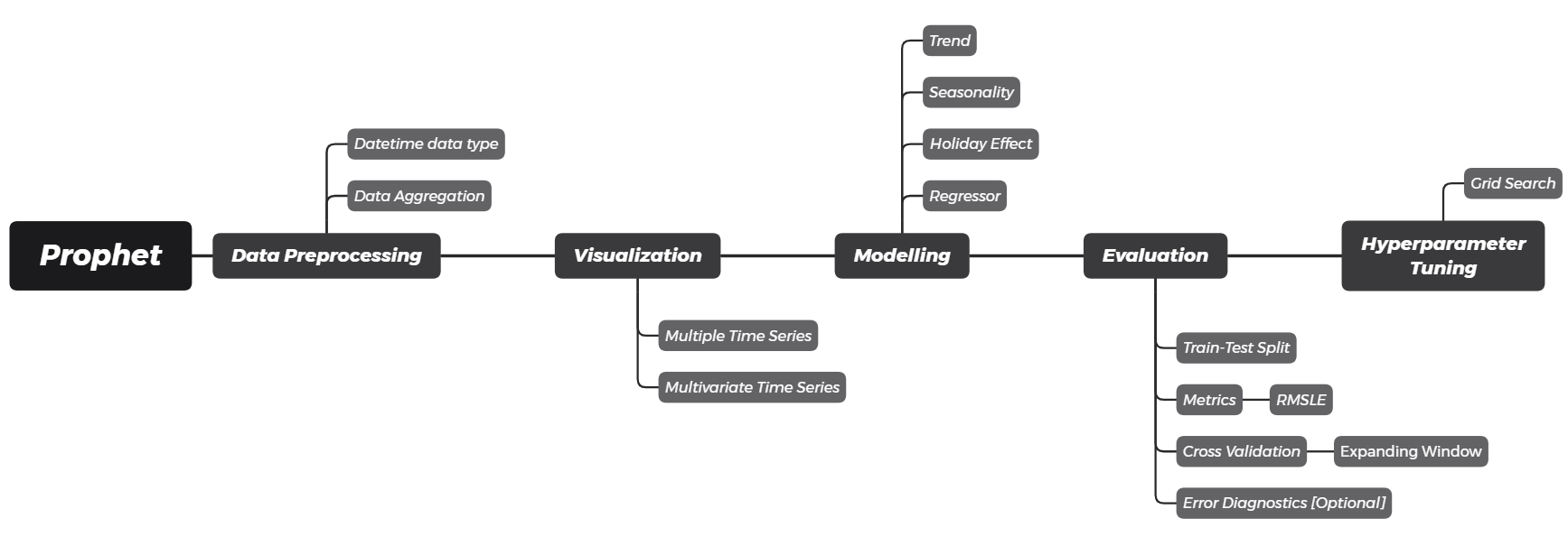
A comprehensive workflow to forecast software sales using the prophet library, provided by Facebook. This post breakdowns each components of time series, including trend, seasonality, holiday effect, and external regressors. The model is then evaluated using RMSLE by expanding window cross validation. Hyperparameter tuning is done using the grid search algorithm.

- Introduction
- Data Loading
- Data Preprocessing
- Visualization
- Modeling using fbprophet
- Forecasting Evaluation
- Hyperparameter Tuning
- Final Forecasting Result
- References
Introduction
Time series data is one of the most common form of data to be found in every industry. It is considered to be a significant area of interest for most industries: retail, telecommunication, logistic, engineering, finance, and socio-economic. Time series analysis aims to extract the underlying components of a time series to better understand the nature of the data. In this post, we will tackle a common industry case of business sales.
import numpy as np
import pandas as pd

# data visualization
import matplotlib.pyplot as plt
import seaborn as sns
import plotly.io as pio

# visualization settings
plt.style.use('seaborn')
plt.rcParams['figure.facecolor'] = 'white'
pio.renderers.default = 'colab'

# prophet
from fbprophet.diagnostics import cross_validation, performance_metrics
from fbprophet.plot import plot_plotly, plot_components_plotly, plot_cross_validation_metric
from fbprophet import Prophet, hdays

# evaluation metric
from sklearn.metrics import mean_squared_log_error

# others
import itertools
from tqdm import tqdm
Data Loading
We will be using provided data from one of the largest Russian software firms - 1C Company and is made available through Kaggle. This is a good example case of data since it contains seasonality and a particular noise in several data when special occurences happened.
sales = pd.read_csv('data_input/sales_train.csv')
sales.head()
The following are the glossary provided in the Kaggle platform:
-
dateis the date format provided in dd.mm.yyyy format -
date_block_numis a consecutive month number used for convenience (January 2013 is 0, February 2013 is 1, and so on) -
shop_idis the unique identifier of the shop -
item_idis the unique identifier of the product -
item_priceis the price of the item on the specified date -
item_cnt_dayis the number of products sold on the specified date
item_cnt_day and item_price, which we’ll see how to analyze the business demand from the sales record.
sales.info()
Some insights we can get from the output are:
- The data consist of 2,935,849 observations (or rows)
- It has 6 variables (or columns)
Data Preprocessing
Time series data is defined as data observations that are collected at regular time intervals. In this case, we are talking about software sales daily data.
We have to make sure our data is ready to be fitted into models, such as:
- Convert
datecolumn data type fromobjecttodatetime64 - Sort the data ascending by
datecolumn - Feature engineering of
total_revenue, which will be forecasted
sales['date'] = pd.to_datetime(sales['date'], dayfirst=True)
sales.sort_values('date', inplace=True)
sales['total_revenue'] = sales['item_price'] * sales['item_cnt_day']
sales.dtypes
pandas will infer date as a month first order by default. Since the sales date is stored in dd.mm.yyyy format, we have to specify parameter dayfirst=True inside pd.to_datetime() method.
Take a look on the third observation below; pandas converts it to 2nd January while the actual data represents February 1st.
date = pd.Series(['30-01-2021', '31-01-2021', '01-02-2021', '02-02-2021'])
pd.to_datetime(date)  # format of datetime64 is yyyy-mm-dd
Next, let's check the date range of sales data. Turns out it ranges from January 1st, 2013 to October 31st, 2015.
sales['date'].apply(['min', 'max'])
We are interested in analyzing the most popular shop (shop_id) of our sales data. The popularity of a shop is defined by the number of transaction that occur. Let's create a frequency table using .value_counts() as follows:
top_3_shop = sales['shop_id'].value_counts().head(3)
top_3_shop
We have gain the information that shop 31, 25, and 54 are the top three shops with the most record sales. Say we would like to analyze their time series attribute. To do that, we can apply conditional subsetting (filter) to sales data.
sales_top_3_shop = sales[sales['shop_id'].isin(top_3_shop.index)]
sales_top_3_shop.head()
Now let’s highlight again the most important definition of a time series:
Now let’s take a look at the codes:
daily_sales = sales_top_3_shop.groupby(['date', 'shop_id'])[['item_cnt_day', 'total_revenue']] \
    .sum().reset_index() \
    .rename(columns={'item_cnt_day': 'total_qty'})
daily_sales.head()
Visualization
One of an important aspect in time series analysis is performing a visual exploratory analysis. Python is known for its graphical capabilities and has a very popular visualization package called matplotlib and seaborn. Let’s take our daily_sales data frame we have created earlier and observe through the visualization.
sns.relplot(data=daily_sales,
            kind='line',
            x='date',
            y='total_qty',
            col='shop_id',
            aspect=6/5)
plt.show()

From the visualization we can conclude that the fluctuation of total_qty is very distinct for each shop. There are some extreme spikes on shop_id 25 and 31 at the end of each year, while shop_id 54 doesn't have any spike.
daily_sales_31 = daily_sales[daily_sales['shop_id'] == 31].reset_index(drop=True)
daily_sales_31.set_index('date')[['total_qty', 'total_revenue']].plot(subplots=True,
                                                                      figsize=(10, 5))
plt.suptitle('DAILY SOFTWARE SALES: STORE 31')
plt.show()

From the visualization we can conclude that the fluctuation of total_qty and total_revenue is quite similar for shop_id 31.
total_qty sold increases, logically, the total_revenue will also increases. We can use total_qty as the regressor when forecasting total_revenue.
Modeling using fbprophet
A very fundamental part in understanding time series is to be able to decompose its underlying components. A classic way in describing a time series is using General Additive Model (GAM). This definition describes time series as a summation of its components. As a starter, we will define time series with 3 different components:
- Trend ($T$): Long term movement in its mean
- Seasonality ($S$): Repeated seasonal effects
- Residuals ($E$): Irregular components or random fluctuations not described by trend and seasonality
The idea of GAM is that each of them is added to describe our time series:
$Y(t) = T(t) + S(t) + E(t)$
Prophet enhanced the classical trend and seasonality components by adding a holiday effect. It will try to model the effects of holidays which occur on some dates and has been proven to be really useful in many cases. Take, for example: Lebaran Season. In Indonesia, it is really common to have an effect on Lebaran season. The effect, however, is a bit different from a classic seasonality effect because it shows the characteristics of an irregular schedule.
Prepare the data
To use the fbprophet package, we first need to prepare our time series data into a specific format data frame required by the package. The data frame requires 2 columns:
-
ds: the time stamp column, stored indatetime64data type -
y: the value to be forecasted
In this example, we will be using the total_qty as the value to be forecasted.
daily_total_qty = daily_sales_31[['date', 'total_qty']].rename(
    columns={'date': 'ds',
             'total_qty': 'y'})

daily_total_qty.head()
model_31 = Prophet()
model_31.fit(daily_total_qty)
Forecasting
Based on the existing data, let's say we would like to perform a forecasting for 1 years into the future. To do that, we will need to first prepare a data frame that consist of the future time stamp range. Conveniently, fbprophet has provided .make_future_dataframe() method that help us to prepare the data:
future_31 = model_31.make_future_dataframe(periods=365, freq='D')
future_31.tail()
Now we have acquired a new future_31 data frame that consist of a date span of the beginning of a time series to 365 days into the future. We will then use this data frame is to perform the forecasting by using .predict() method of our model_31:
forecast_31 = model_31.predict(future_31)
forecast_31[['ds', 'trend', 'weekly', 'yearly', 'yhat']]
Recall that in General Additive Model, we use time series components and perform a summation of all components. In this case, we can see that the model is extracting 3 types of components: trend, weekly seasonality, and yearly seasonality. Means, in forecasting future values it will use the following formula: $yhat(t) = T(t) + S_{weekly}(t) + S_{yearly}(t)$
We can manually confirm from forecast_31 that the column yhat is equal to trend + weekly + yearly.
forecast_result = forecast_31['yhat']
forecast_add_components = forecast_31['trend'] + forecast_31['weekly'] + forecast_31['yearly']

(forecast_result.round(10) == forecast_add_components.round(10)).all()
.round() is performed to prevent floating point overflow.
Visualize
Now, observe how .plot() method take our model_31, and newly created forecast_31 object to create a matplotlib object that shows the forecasting result. The black points in the plot shows the actual time series, and the blue line shows the fitted time series along with its forecasted values 365 days into the future.
fig = model_31.plot(forecast_31, xlabel='Date', ylabel='Quantity Sold')

We can also visualize each of the trend and seasonality components using .plot_components method.
fig = model_31.plot_components(forecast_31)

From the visualization above, we can get insights such as:
- The trend shows that the
total_qtysold is decreasing from time to time. - The weekly seasonality shows that sales on weekends are higher than weekdays.
- The yearly seasonality shows that sales peaked at the end of the year.
plotly 4.0 or above separately, as it will not by default be installed with fbprophet. You will also need to install the notebook and ipywidgets packages.
plot_plotly(model_31, forecast_31)
plot_components_plotly(model_31, forecast_31)
# for illustration purposes only
from datetime import date

# prepare data
daily_sales_31_copy = daily_sales_31.copy()
daily_sales_31_copy['date_ordinal'] = daily_sales_31_copy['date'].apply(lambda date: date.toordinal())

# visualize regression line
plt.figure(figsize=(10, 5))
ax = sns.regplot(x='date_ordinal',
                 y='total_qty',
                 data=daily_sales_31_copy,
                 scatter_kws={'color': 'black', 's': 2},
                 line_kws={'color': 'red'})
new_labels = [date.fromordinal(int(item)) for item in ax.get_xticks()]
ax.set_xticklabels(new_labels)
plt.xlabel('date')
plt.show()

Automatic Changepoint Detection
Prophet however implements a changepoint detection which tries to automatically detect a point where the slope has a significant change rate. It will tries to split the series using several points where the trend slope is calculated for each range.
prophet specifies 25 potential changepoints (n_changepoints=25) which are placed uniformly on the first 80% of the time series (changepoint_range=0.8).
# for illustration purposes only
from fbprophet.plot import add_changepoints_to_plot
fig = model_31.plot(forecast_31, xlabel='Date', ylabel='Quantity Sold')
a = add_changepoints_to_plot(fig.gca(), model_31, forecast_31, threshold=0)

From the 25 potential changepoints, it will then calculate the magnitude of the slope change rate and decided the significant change rate. The model detected 3 significant changepoints and separate the series into 4 different trend slopes.
fig = model_31.plot(forecast_31, xlabel='Date', ylabel='Quantity Sold')
a = add_changepoints_to_plot(fig.gca(), model_31, forecast_31)

Adjusting Trend Flexibility
Prophet provided us a tuning parameter to adjust the detection flexibility:
-
n_changepoints(default = 25): The number of potential changepoints, not recommended to be tuned, this is better tuned by adjusting the regularization (changepoint_prior_scale) -
changepoint_range(default = 0.8): Proportion of the history in which the trend is allowed to change. Recommended range: [0.8, 0.95] -
changepoint_prior_scale(default = 0.05): The flexibility of the trend, and in particular how much the trend changes at the trend changepoints. Recommended range: [0.001, 0.5]
model_tuning_trend = Prophet(
    n_changepoints=25,  # default = 25
    changepoint_range=0.8,  # default = 0.8
    changepoint_prior_scale=0.5  # default = 0.05
)
model_tuning_trend.fit(daily_total_qty)

# forecasting
future = model_tuning_trend.make_future_dataframe(periods=365, freq='D')
forecast = model_tuning_trend.predict(future)

# visualize
fig = model_tuning_trend.plot(forecast, xlabel='Date', ylabel='Quantity Sold')
a = add_changepoints_to_plot(fig.gca(), model_tuning_trend, forecast)

fig = model_31.plot_components(forecast_31)
By default, Prophet will try to determine existing seasonality based on existing data provided. In our case, the data provided is a daily data from early 2013 to end 2015.
- Any daily sampled data by default will be detected to have a weekly seasonality.
- While yearly seasonality, by default will be set as
Trueif the provided data has more than 2 years of daily sample. - The other regular seasonality is a daily seasonality which tries to model an hourly pattern of a time series. Since our data does not accommodate hourly data, by default the daily seasonality will be set as
False.
model_tuning_seasonality = Prophet(
    weekly_seasonality=3,  # default = 3
    yearly_seasonality=200  # default = 10
)
model_tuning_seasonality.fit(daily_total_qty)

# forecasting
future = model_tuning_seasonality.make_future_dataframe(periods=365, freq='D')
forecast = model_tuning_seasonality.predict(future)

# visualize
fig = model_tuning_seasonality.plot_components(forecast)

Custom Seasonalities
The default provided seasonality modelled by Prophet for a daily sampled data is: weekly and yearly.
Consider this case: a sales in your business is heavily affected by payday. Most customers tends to buy your product based on the day of the month. Since it did not follow the default seasonality of yearly and weekly, we will need to define a non-regular seasonality. There are two steps we have to do:
- Remove default seasonality (eg: remove yearly seasonality) by setting
False - Add seasonality (eg: add monthly seasonality) by using
.add_seasonality()method before fitting the model
We ended up with formula: $yhat(t) = T(t) + S_{weekly}(t) + \bf{S_{monthly}(t)}$
model_custom_seasonality = Prophet(
    yearly_seasonality=False  # remove seasonality
)
# add seasonality
model_custom_seasonality.add_seasonality(
    name='monthly', period=30.5, fourier_order=5)
model_custom_seasonality.fit(daily_total_qty)

# forecasting
future = model_custom_seasonality.make_future_dataframe(periods=365, freq='D')
forecast = model_custom_seasonality.predict(future)

# visualize
fig = model_custom_seasonality.plot_components(forecast)

For monthly seasonality, we provided period = 30.5 indicating that there will be non-regular 30.5 frequency in one season of the data. The 30.5 is a common frequency quantifier for monthly seasonality, since there are some months with a total of 30 and 31 (some are 28 or 29).
fig = model_31.plot(forecast_31, xlabel='Date', ylabel='Quantity Sold')
plt.axhline(y=800, color='red', ls='--')
plt.show()

Table below shows that the relatively large sales mostly happened at the very end of a year between 27th to 31st December. Now let’s assume that this phenomenon is the result of the new year eve where most people spent the remaining budget of their Christmas or End year bonus to buy our goods.
daily_total_qty[daily_total_qty['y'] > 800]
We'll need to prepare a holiday data frame with the following column:
-
holiday: the holiday unique name identifier -
ds: timestamp -
lower_window: how many time unit behind the holiday that is assumed to to be affected (smaller or equal than zero) -
upper_window: how many time unit after the holiday that is assumed to be affected (larger or equal to zero)
holiday = pd.DataFrame({
    'holiday': 'new_year_eve',
    'ds': pd.to_datetime(['2013-12-31', '2014-12-31',  # past date, historical data
                          '2015-12-31']),  # future date, to be forecasted
    'lower_window': -4,  # include 27th - 31st December
    'upper_window': 0})
holiday
Once we have prepared our holiday data frame, we can pass that into the Prophet() class:
model_holiday = Prophet(holidays=holiday)
model_holiday.fit(daily_total_qty)

# forecasting
future = model_holiday.make_future_dataframe(periods=365, freq='D')
forecast = model_holiday.predict(future)

# visualize
fig = model_holiday.plot(forecast, xlabel='Date', ylabel='Quantity Sold')

Now, observe how it has more confidence in capturing the holiday effect on the end of the year instead of relying on the yearly seasonality effect. If we plot the components, we could also get the holiday components listed as one of the time series components:
fig = model_holiday.plot_components(forecast)

model_holiday_indo = Prophet()
model_holiday_indo.add_country_holidays(country_name='ID')
model_holiday_indo.fit(daily_total_qty)

model_holiday_indo.train_holiday_names
hdays module. This is useful if we want to take a look on the holiday dates and then manually include only certain holidays.
# Reference code: https://github.com/facebook/prophet/blob/master/python/fbprophet/hdays.py
holidays_indo = hdays.Indonesia()
holidays_indo._populate(2021)
pd.DataFrame([holidays_indo], index=['holiday']).T.rename_axis('ds').reset_index()
Adding Regressors
Additional regressors can be added to the linear part of the model using the .add_regressor() method, before fitting model. In this case, we want to forecast total_revenue based on its previous revenue components (trend, seasonality, holiday) and also total_qty sold as the regressor:
$revenue(t) = T_{revenue}(t) + S_{revenue}(t) + H_{revenue}(t) + \bf{qty(t)}$
model_total_qty = Prophet(
    n_changepoints=20,  # trend flexibility
    changepoint_range=0.9,  # trend flexibility
    changepoint_prior_scale=0.25,  # trend flexibility
    weekly_seasonality=5,  # seasonality fourier order
    yearly_seasonality=False,  # remove seasonality
    holidays=holiday  # new year eve effects
)
# add monthly seasonality
model_total_qty.add_seasonality(name='monthly', period=30.5, fourier_order=5)
model_total_qty.fit(daily_total_qty)

# forecasting
future = model_total_qty.make_future_dataframe(periods=365, freq='D')
forecast_total_qty = model_total_qty.predict(future)

# visualize
fig = model_total_qty.plot(
    forecast_total_qty, xlabel='Date', ylabel='Quantity Sold')

The table below shows the forecasted total quantity for the last 365 days (from November 1st, 2015 until October 30th, 2016).
forecasted_total_qty = forecast_total_qty[['ds', 'yhat']].tail(365) \
    .rename(columns={'yhat': 'total_qty'})
forecasted_total_qty
On the other hand, the table below shows the actual total quantity which we used for training model. We have to rename the column exactly like the previous table.
actual_total_qty = daily_total_qty.rename(columns={'y': 'total_qty'})
actual_total_qty
Now, we have to prepare concatenated data of total_qty as the regressor values of total_revenue:
- First 1031 observations: actual values of
total_qty - Last 365 observations: forecasted values of
total_qty
future_with_regressor = pd.concat([actual_total_qty, forecasted_total_qty])
future_with_regressor
daily_total_revenue = daily_sales_31[['date', 'total_revenue', 'total_qty']].rename(
    columns={'date': 'ds',
             'total_revenue': 'y'})

daily_total_revenue.head()
During fitting a model with regressor, make sure:
- Apply
.add_regressor()method before fitting - Forecast the value using
future_with_regressordata frame that we have prepared before, containingdsand the regressor values
model_total_revenue = Prophet(
    holidays=holiday  # new year eve effects
)
# add regressor
model_total_revenue.add_regressor('total_qty')
model_total_revenue.fit(daily_total_revenue)

# forecasting
# use dataframe with regressor, instead of just `ds` column
forecast_total_revenue = model_total_revenue.predict(future_with_regressor)

# visualize
fig = model_total_revenue.plot(
    forecast_total_revenue, xlabel='Date', ylabel='Total Revenue')

If we plot the components, we could also get the extra regressors components listed as one of the time series components:
fig = model_total_revenue.plot_components(forecast_total_revenue)

Forecasting Evaluation
Recall how we performed a visual analysis on how the performance of our forecasting model earlier. The technique was in fact, a widely used technique for model cross-validation. It involves splitting our data into two parts:
- Train data is used to train our time series model in order to acquire the underlying patterns such as trend and seasonality.
- Test data is purposely being kept for us to perform a cross-validation and see how our model perform on an unseen data.
cutoff = pd.to_datetime('2015-01-01')
daily_total_qty['type'] = daily_total_qty['ds'].apply(
    lambda date: 'train' if date < cutoff else 'test')

plt.figure(figsize=(10, 5))
sns.scatterplot(x='ds', y='y', hue='type', s=5,
                palette=['black', 'red'],
                data=daily_total_qty)
plt.axvline(x=cutoff, color='gray', label='cutoff')
plt.legend()
plt.show()

We can split at a cutoff using conditional subsetting as below:
train = daily_total_qty[daily_total_qty['ds'] < cutoff]
test = daily_total_qty[daily_total_qty['ds'] >= cutoff]

print(f'Train length: {train.shape[0]} days')
print(f'Test length: {test.shape[0]} days')
Now let's train the model using data from 2013-2014 only, and forecast 303 days into the future (until October 31st, 2015).
model_final = Prophet(
    holidays=holiday,  # holiday effect
    yearly_seasonality=True)
# add monthly seasonality
model_final.add_seasonality(name='monthly', period=30.5, fourier_order=5)
model_final.fit(train)  # only training set

# forecasting
future_final = model_final.make_future_dataframe(
    periods=303, freq='D')  # 303 days (test size)
forecast_final = model_final.predict(future_final)

# visualize
fig = model_final.plot(forecast_final, xlabel='Date', ylabel='Quantity Sold')
plt.scatter(x=test['ds'], y=test['y'], s=10, color='red')
plt.show()

Evaluation Metrics
Based on the plot above, we can see that the model is capable in forecasting the actual future value. But for most part, we will need to quantify the error to be able to have a conclusive result. To quantify an error, we need to calculate the difference between actual demand and the forecasted demand. However, there are several metrics we can use to express the value. Some of them are:
- Root Mean Squared Error
- Root Mean Squared Logarithmic Error
Notation:
- $n$: length of time series
- $p_i$: predicted value at time $i$
- $a_i$: actual value at time $i$
# for illustration purposes only

# calculation
err = np.arange(-500, 500)
p = np.arange(0, 1000)
a = p - err
rmse_plot = np.power(err, 2) ** 0.5
rmsle_plot = np.power(np.log1p(p) - np.log1p(a), 2) ** 0.5

# visualization
fig, axes = plt.subplots(1, 2, figsize=(12, 5))

for idx, (ax, y) in enumerate(zip(axes, [rmse_plot, rmsle_plot])):
    ax.plot(err[err < 0], y[err < 0], color='red', label="Underestimate")
    ax.plot(err[err > 0], y[err > 0], color='blue', label="Overestimate")
    ax.set_xlabel("Error (Prediction - Actual)")
    ax.set_ylabel(f"RMS{'L' if idx else ''}E")
    ax.set_title(f"Root Mean Squared {'Logarithmic ' if idx else ''}Error")
    ax.legend()

plt.show()

forecast_train = forecast_final[forecast_final['ds'] < cutoff]
train_rmsle = mean_squared_log_error(y_true=train['y'],
                                     y_pred=forecast_train['yhat']) ** 0.5
train_rmsle
forecast_test = forecast_final[forecast_final['ds'] >= cutoff]
test_rmsle = mean_squared_log_error(y_true=test['y'],
                                    y_pred=forecast_test['yhat']) ** 0.5
test_rmsle
Expanding Window Cross Validation
Instead of only doing one time train-test split, we can do cross validation as shown below:
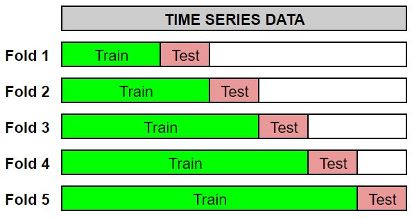
This cross validation procedure is called as expanding window and can be done automatically by using the cross_validation() method. There are three parameters to be specified:
-
initial: the length of the initial training period -
horizon: forecast length -
period: spacing between cutoff dates
df_cv = cross_validation(model_total_revenue, initial='730 days', horizon='30 days', period='90 days')
df_cv
The cross validation process above will be carried out for 4 folds, where at each fold a forecast will be made for the next 30 days (horizon) from the cutoff dates. Below is the illustration for each fold:
# for illustration purposes only
df_copy = daily_total_qty[['ds', 'y']].copy()
df_cutoff_horizon = df_cv.groupby('cutoff')[['ds']].max()

for i, (cutoff, horizon) in enumerate(df_cutoff_horizon.iterrows()):
    horizon_cutoff = horizon['ds']

    df_copy['type'] = df_copy['ds'].apply(
        lambda date: 'train' if date < cutoff else
                     'test' if date < horizon_cutoff else 'unseen')

    plt.figure(figsize=(10, 5))
    sns.scatterplot(x='ds', y='y', hue='type', s=5,
                    palette=['black', 'red', 'gray'],
                    data=df_copy)
    plt.axvline(x=cutoff, color='gray', label='cutoff')
    plt.axvline(x=horizon_cutoff, color='gray', ls='--', label='horizon')
    plt.legend(bbox_to_anchor=(1, 1), loc='upper left')
    plt.title(
        f"FOLD {i+1}\nTRAIN SIZE: {df_copy['type'].value_counts()['train']} DAYS")
    plt.show()


Cross validation error metrics can be evaluated for each folds, here shown for RMSLE.
cv_rmsle = df_cv.groupby('cutoff').apply(
    lambda x: mean_squared_log_error(y_true=x['y'],
                                     y_pred=x['yhat']) ** 0.5)
cv_rmsle
We can aggregate the metrics by using its mean. In other words, we are calculating the mean of RMSLE to represent the overall model performance.
cv_rmsle.mean()
Error Diagnostics
Prophet has provide us several frequently used evaluation metrics by using performance_metrics():
- Mean Squared Error (MSE)
- Root Mean Squared Error (RMSE)
- Mean Absolute Error (MAE)
- Mean Absolute Percentage Error (MAPE)
- Median Absolute Percentage Error (MDAPE)
- Coverage: Percentage of actual data that falls on the forecasted uncertainty (confidence) interval
df_p = performance_metrics(df_cv, rolling_window=0)
df_p.tail()
Cross validation performance metrics can be visualized with plot_cross_validation_metric, here shown for RMSE.
- Dots show the root squared error (RSE) for each prediction in
df_cv. - The blue line shows the RMSE for each horizon.
fig = plot_cross_validation_metric(df_cv, metric='rmse', rolling_window=0)

sklearn.metrics module.
- Dots show the root squared logarithmic error (RSLE) for each prediction in
df_cv. - The blue line shows the RMSLE for each horizon.
# calculation
df_cv['horizon'] = (df_cv['ds'] - df_cv['cutoff']).dt.days
df_cv['sle'] = np.power((np.log1p(df_cv['yhat']) - np.log1p(df_cv['y'])), 2) # squared logarithmic error
df_cv['rsle'] = df_cv['sle'] ** 0.5
horizon_rmsle = df_cv.groupby('horizon')['sle'].apply(lambda x: x.mean() ** 0.5) # root mean

# visualization
plt.figure(figsize=(10, 5))
sns.scatterplot(x='horizon', y='rsle',
                s=15, color='gray',
                data=df_cv)
plt.plot(horizon_rmsle.index, horizon_rmsle, color='blue')
plt.grid(b=True, which='major', color='gray', linestyle='-')
plt.xlabel('Horizon (days)')
plt.ylabel('RMSLE')
plt.show()

Hyperparameter Tuning
In this section, we implement a Grid search algorithm for model tuning by using for-loop. It builds model for every combination from specified hyperparameters and then evaluate it. The goal is to choose a set of optimal hyperparameters which minimize the forecast error (in this case, smallest RMSLE).
param_grid = {
    'changepoint_prior_scale': [0.001, 0.01, 0.1],
    'changepoint_range': [0.8, 0.95]
}

# Generate all combinations of parameters
all_params = [dict(zip(param_grid.keys(), v))
              for v in itertools.product(*param_grid.values())]
rmsles = []  # Store the RMSLEs for each params here

# Use cross validation to evaluate all parameters
for params in tqdm(all_params):
    # fitting model
    # (TO DO: change the data and add other components: seasonality, holiday, regressor)
    model = Prophet(**params,
                    holidays=holiday)
    model.fit(daily_total_qty)

    # Expanding window cross validation (TO DO: use different values)
    cv = cross_validation(model, initial='730 days', period='90 days', horizon='60 days',
                          parallel='processes')

    # Evaluation metrics: RMSLE
    rmsle = cv.groupby('cutoff').apply(
        lambda x: mean_squared_log_error(y_true=x['y'],
                                         y_pred=x['yhat']) ** 0.5)

    mean_rmsle = rmsle.mean()
    rmsles.append(mean_rmsle)
daily_total_qty for the sake of explanation simplicity.
We can observe the error metrics for each hyperparameter combination, and sort by ascending:
tuning_results = pd.DataFrame(all_params)
tuning_results['rmsle'] = rmsles
tuning_results.sort_values(by='rmsle')
Best hyperparameter combination can be extracted as follows:
best_params = all_params[np.argmin(rmsles)]
best_params
Lastly, re-fit the model and use it for forecasting.
model_best = Prophet(**best_params, holidays=holiday)
model_best.fit(daily_total_qty)
model_best
** is an operator for dictionary unpacking. It delivers key-value pairs in a dictionary into a function’s arguments.
future_best = model_best.make_future_dataframe(periods=365, freq='D')
forecast_best = model_best.predict(future_best)

# visualize
fig = model_best.plot(forecast_best, xlabel='Date', ylabel='Quantity Sold')

The final forecasting result then can be used as a sales target for one year ahead.