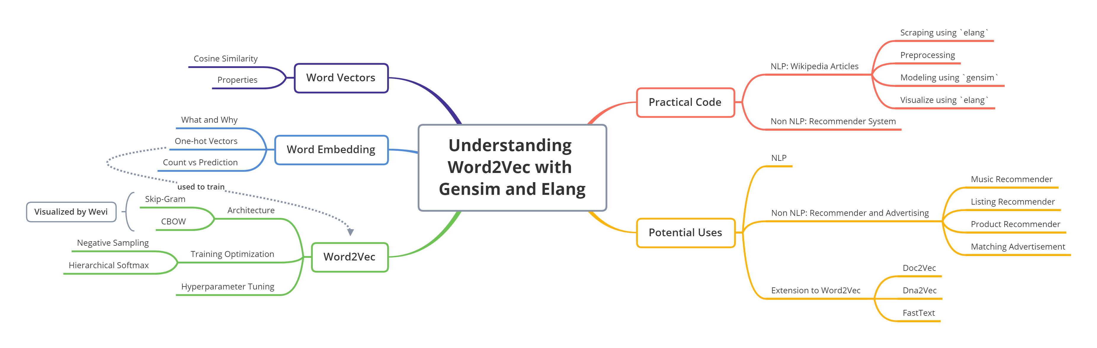
Understanding Word2Vec with Gensim and Elang
A comprehensive material on Word2Vec, a prediction-based word embeddings developed by Tomas Mikolov (Google). The explanation begins with the drawbacks of word embedding, such as one-hot vectors and count-based embedding. Word vectors produced by the prediction-based embedding have interesting properties that can capture the semantic meaning of a word. Therefore, we are interested in deep dive the Word2Vec in terms of its architecture, training optimization method, and how to do the hyperparameter tuning. We also tried to create Word2Vec embedding from scraped Wikipedia articles with the help of gensim and visualized it using elang - a Python package developed by Samuel Chan and me. We also present some other non-NLP use cases and developments from Word2Vec. At the end of this post, there are five multiple choice questions to test your understanding.

- Packages
- Introduction to Word Embedding
- Word Vectors Intuition
- Word2Vec
- Practical Word2Vec using Gensim and Elang on Wikipedia Articles
- Potential Uses
- Test Your Understanding!
- References
Next, we create a connection between Google Colab and Drive. Please go through the authentication step then download the file using the Google File ID.
from pydrive.auth import GoogleAuth
from pydrive.drive import GoogleDrive
from google.colab import auth
from oauth2client.client import GoogleCredentials

auth.authenticate_user()
gauth = GoogleAuth()
gauth.credentials = GoogleCredentials.get_application_default()
drive = GoogleDrive(gauth)
# you can replace the id with id of file you want to access
model_id = "1vXsf0DI8HKGuqYFIGIrvG-73KzZPgz5h"
downloaded = drive.CreateFile({'id':model_id})
downloaded.GetContentFile('wiki_Animal.model')
Import necessary Python packages for the content.
import pandas as pd
import numpy as np

# text processing
import nltk
nltk.download(["brown", "stopwords"])
from nltk.corpus import brown
from nltk.probability import FreqDist

# visualization
import matplotlib.pyplot as plt

# other packages
from itertools import combinations
from tqdm import tqdm

import warnings
warnings.filterwarnings('ignore')
What does it mean?
Word embedding is one of the most popular representation of document vocabulary. It is capable of capturing context of a word in a document, semantic and syntactic similarity, relation with other words, etc. It is just a fancy way of saying numerical representation of words. A good analogy would be how we use the RGB representation for colors.
Why do we need them?
As a human, it doesn’t make much sense in wanting to represent words using numbers because numbers are used for quantification and why would one need to quantify words?
The answer to that is, we want to quantify the semantics. We want to represent words in such a manner that it captures its meaning in a way humans do. Not the exact meaning of the word but a contextual one. For example, when I say the word "see", we know exactly what action — the context — I’m talking about, even though we might not be able to quote its meaning, the kind we would find in a dictionary, of the top of our head.
One-hot Vectors
The simplest word embedding you can have is using one-hot vectors. If you have $n$ words in your vocabulary, then you can represent each word as a $1 \times n$ vector.
For a simple example, if we have 3 words — dog, cat, hat — in our vocabulary then we can represent them as following:
dog [1, 0, 0]
cat [0, 1, 0]
hat [0, 0, 1]
Problems:
- Curse of dimensionality: Size of vectors depends on the size of our vocabulary (which can be huge). This is a wastage of space and increases algorithm complexity exponentially.
- Transfer learning would be impossible if we add/remove words from the vocabulary, as it would require to re-train the whole model again.
- This representation fails to capture the contextual meaning of the words. There is no correlation between words that have similar meaning or usage.
Using one-hot vectors, Similarity(dog, cat) == Similarity(dog, hat) == 0. But in an ideal situation, Similarity(dog, cat) >> Similarity(dog, hat)
Count-based Embedding
This is one type of word embeddings, based on the count of each words. One of them is a count vector.
Count Vector
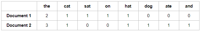
Count vector model learns a vocabulary from all of the documents, then models each document by counting the number of times each word appears. For example, consider we have $D$ documents and $T$ is the number of different words in our vocabulary then the size of count vector matrix will be given by $D \times T$. Let’s take the following two sentences:
Document 1: "The cat sat on the hat"
Document 2: "The dog ate the cat and the hat"
then the count vector matrix is:
The Drawback
Count-based language modeling is easy to comprehend — related words are observed (counted) together more often than unrelated words. Many attempts were made to improve the performance of the model to the state-of-art, using SVD, ramped window, and non-negative matrix factorization, but the model did not do well in capturing complex relationships among words.
Then, the paradigm started to change in 2013, when Thomas Mikolov proposed the prediction-based modeling technique, called Word2Vec. Unlike counting word co-occurrences, the model uses neural networks to learn intelligent representation of words in a vector space. Then, the paper Don’t count, predict! A systematic comparison of context-counting vs. context-predicting semantic vectors, quantified & compared the performances of count-based vs prediction-based models.
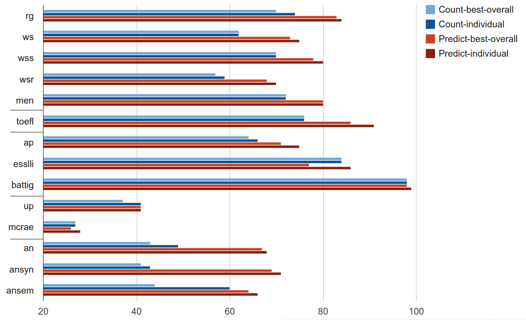
The blue bars represent the count-based models, and the red bars are for prediction-based models. Long story short, prediction-based models outperformed count-based models by a large margin on various language tasks.
Word Vectors Intuition
Consider a small subset of English: words for animals. Our task is to be able to write computer programs to find similarities among these words and the creatures they designate. To do this, we might start by making a spreadsheet of some animals and their characteristics. For example:
animal = pd.DataFrame({
    "animal": ["kitten", "hamster", "tarantula", "puppy", "crocodile", "dolphin", "panda bear", "lobster", "capybara", "elephant", "mosquito", "goldfish", "horse", "chicken"],
    "cuteness": [95, 80, 8, 90, 5, 60, 75, 2, 70, 65, 1, 25, 50, 25],
    "size": [15, 8, 3, 20, 40, 45, 40, 15, 30, 90, 1, 2, 50, 15]
}).set_index("animal")
animal
Euclidean Distance vs Cosine Similarity
DataFrame animals give us information we need to make determinations about which animals are similar (at least, similar in the properties that we've included in the data). Try to answer the following question: Which animal is most similar to a capybara?

You could go through the values one by one and do the math to make that evaluation, but visualizing the data as points in 2-dimensional space makes finding the answer very intuitive:
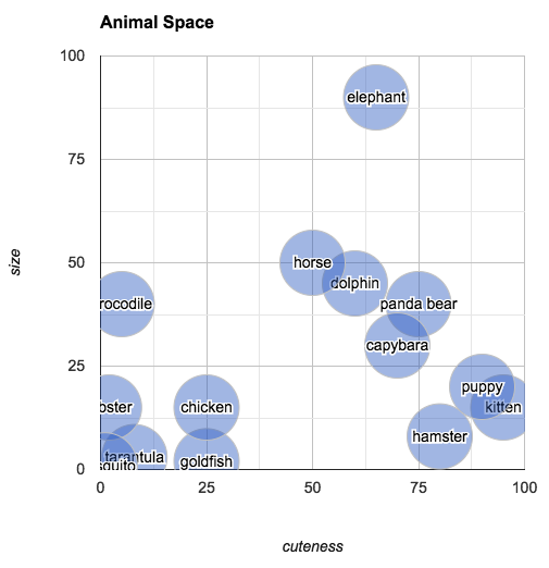
The plot shows us that the closest animal to the capybara is the panda bear (in terms of its subjective size and cuteness). One way of calculating how "far apart" two points are is to find their Euclidean distance.
Using Euclidean distance might be fine for a lower dimension, how about we contrast it with this case:
Let's say you are in an e-commerce setting and you want to compare users for product recommendations.
User 1 bought 1x eggs, 1x flour, and 1x sugar
User 2 bought 100x eggs, 100x flour, and 100x sugar
User 3 bought 1x sugar, 1x Vodka, and 1x Red Bull
purchase = pd.DataFrame({
"user": ["user 1", "user 2", "user 3"],
"eggs": [1, 100, 0],
"flour": [1, 100, 0],
"sugar": [1, 100, 1],
"vodka": [0, 0, 1],
"red bull": [0, 0, 1]
}).set_index("user")
purchase
for a, b in combinations(purchase.index, 2):
    dist = np.linalg.norm(purchase.loc[a]-purchase.loc[b])
    print(f"Euclidean Distance ({a}, {b}): {dist}")
Problem occurs when we use Euclidean distance, user 3 is more similar to user 1. In fact, user 2 is more similar to user 1 in terms of purchase behavior. The solution is to use Cosine Similarity.
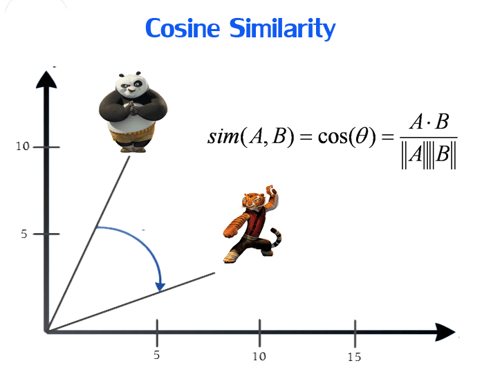
Mathematically, it measures the cosine of the angle between two vectors projected in a multi-dimensional space. Word vectors with similar context occupy close spatial positions; the cosine of the angle between such vectors should be close to 1, i.e. angle close to 0. The smaller the angle, higher the cosine similarity.
def cosine_similarity(x, y):
    dot_products = np.dot(x, y.T)
    norm_products = np.linalg.norm(x) * np.linalg.norm(y)
    return dot_products / norm_products


for a, b in combinations(purchase.index, 2):
    sim = cosine_similarity(purchase.loc[a], purchase.loc[b])
    print(f"Cosine Similarity ({a}, {b}): {sim}")
Interesting Properties
Back to our original illustration:
Modeling animals in this way has a few other interesting properties:
- Most Similar Point
We can pick an arbitrary point in "animal space" and then find the animal closest to that point. If you imagine an animal of size 25 and cuteness 30, you can easily look at the space to find the animal that most closely fits that description: the chicken.
- Average Point
Reasoning visually, you can also answer questions like "what's halfway between a chicken and an elephant?" Simply draw a line from "elephant" to "chicken," mark off the midpoint and find the closest animal. According to our chart, halfway between an elephant and a chicken is a horse.
- Analogous relationship
You can also ask: what's the difference between a hamster and a tarantula? According to our plot, it's about seventy five units of cute (and a few units of size). The relationship of "difference" is an interesting one, because it allows us to reason about analogous relationships. In the chart below, I've drawn an arrow from "tarantula" to "hamster" (in blue):
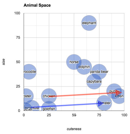
You can understand this arrow as being the relationship between a tarantula and a hamster, in terms of their size and cuteness (i.e., hamsters and tarantulas are about the same size, but hamsters are much cuter). In the same diagram, I've also transposed this same arrow (this time in red) so that its origin point is "chicken." The arrow ends closest to "kitten." What we've discovered is that the animal that is about the same size as a chicken but much cuter is... a kitten. To put it in terms of an analogy:
Tarantulas are to hamsters as chickens are to kittens.
General Architecture
Word2Vec is one of the most popular technique to learn word embeddings using shallow neural network. It was developed by Tomas Mikolov in 2013 at Google.
A prerequisite for any neural network or any supervised training technique is to have labeled training data. How do you a train a neural network to predict word embedding when you don’t have any labeled data i.e words and their corresponding word embedding?
We’ll do that by creating a so-called “fake” task for the neural network to train. We won’t be interested in the inputs and outputs of this network, rather the goal is actually just to learn the weights of the hidden layer that are actually the “word vectors” that we’re trying to learn.
Let us look deeper into the Word2Vec architecture:
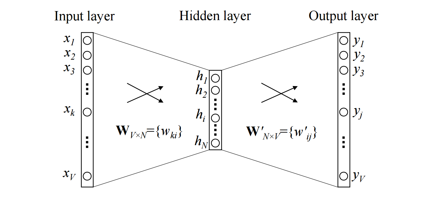
Details:
- The input layer is a one hot encoded vector of size $V$ (vocabulary size).
- $W_{V \times N}$ is the weight matrix that projects the input $x$ to the hidden layer. These values are the word vectors.
- The hidden layer contains $N$ neurons (hyperparameter), it just copy the weighted sum of inputs to the next layer. There is no activation function like sigmoid, tanh or ReLU.
- $W'_{N \times V}$ is the weight matrix that maps the hidden layer outputs to the final output layer.
- The output layer is again a $V$ length vector, with softmax activation function which is a function that turn numbers, aka logits, into probabilities that sum to one.
There are two flavors of Word2Vec in which both are using the same architecture: Skip-Gram and Continuous Bag-Of-Words (CBOW). For each of them, we will be considering this example:
Let's say we have a sentence:
I love to drink orange juice
and we want to generate the training samples for the input and output words with window size is equal to 2. The illustration of sliding window is given by the picture below.
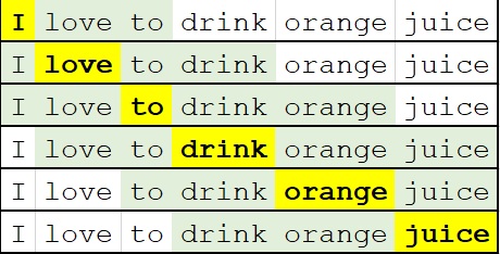
The word highlighted in yellow is the target/center word and the words highlighted in green are its context/neighboring words.
Skip-Gram
Skip-Gram Training Samples
The fake task for Skip-gram model would be: Given a target word, we’ll try to predict its context words. Here are the list of training samples generated from source text if we use skip-gram:
('I', 'love'),
('I', 'to'),

('love', 'I'),
('love', 'to'),
('love', 'drink'),

('to', 'I'),
('to', 'love'),
('to', 'drink'),
('to', 'orange'),

('drink', 'love'),
('drink', 'to'),
('drink', 'orange'),
('drink', 'juice'),

('orange', 'to'),
('orange', 'drink'),
('orange', 'juice'),

('juice', 'drink'),
('juice', 'orange')
Skip-Gram Architecture
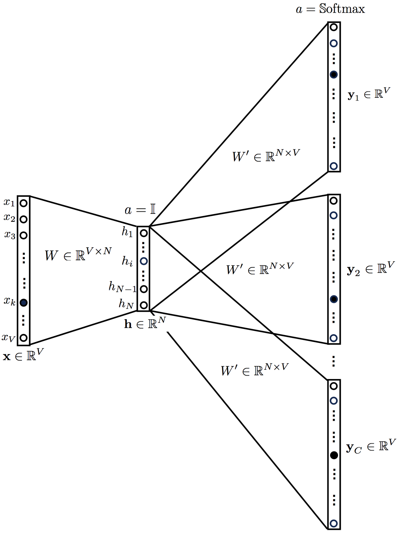
We breakdown the way this model works in these steps:
- Convert the generated training samples into one hot vectors $x$ (center word) for the input layer and $y_1, y_2, ..., y_C$ (context words) for the output, where each is a vector of $V$-dimension.
- Multiply input layer with $W_{V \times N}$ to get the embedded vectors of size $N$.
- The embedded vectors is then multiplied with $W'_{N \times V}$ to get the logit scores of size $V$.
- Apply softmax function to turn the scores into probabilities, we get $\hat{y}$.
- Error between output and each context word is calculated as follows: $\sum \limits_{i=1}^C {(\hat{y} - y_i)}$
- Backpropagation to re-adjust the weights, by using Gradient Descent or other optimizer.
a. All weights in output matrix will be updated.
b. Only corresponding word vector in the input matrix that will be updated.
Continuous Bag-Of-Words (CBOW)
CBOW Training Samples
The fake task in CBOW is somewhat similar to Skip-gram, in the sense that we still take a pair of words and teach the model that they co-occur but instead it is learning to predict the target word by the context words.
('love', 'I'),
('to', 'I'),

('I', 'love'),
('to', 'love'),
('drink', 'love'),

('I', 'to'),
('love', 'to'),
('drink', 'to'),
('orange', 'to'),

('love', 'drink'),
('to', 'drink'),
('orange', 'drink'),
('juice', 'drink'),

('to', 'orange'),
('drink', 'orange'),
('juice', 'orange'),

('drink', 'juice'),
('orange', 'juice')
CBOW Architecture
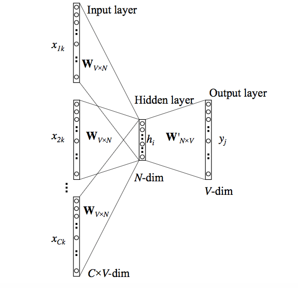
We breakdown the way this model works in these steps:
- Convert the generated training samples into one hot vectors $x_1, x_2, ..., x_C$ (context word) for the input layer. So, the size is $C \times V$
- Multiply all vector $x$ with $W_{V \times N}$ and then take the sum or mean of embedded vectors.
- The hidden layer is then multiplied with $W'_{N \times V}$ to get the logit scores of size $V$.
- Apply softmax function to turn the scores into probabilities, we get $\hat{y}$.
- Error between output and each context word is calculated as follows: ${(\hat{y} - y)}$
- Back-propagation to re-adjust the weights, by using Gradient Descent or other optimizer. Just like Skip-gram:
a. All weights in output matrix will be updated.
b. Only corresponding word vector in the input matrix that will be updated.
def wevi_input(sentence, window=2, sg=1):
    sentence_list = sentence.split()
    result = []
    for idx, target in enumerate(sentence_list):
        context = []
        for w in range(idx-window, idx+window+1):
            if w < 0 or w == idx:
                continue
            try:
                context.append(sentence_list[w])
            except:
                continue
        if sg:
            # Skip-gram
            result.append(target + '|' + '^'.join(context))
        else:
            # CBOW
            result.append('^'.join(context) + '|' + target)
    return ','.join(result)


# specify input
sentences_list = ["I love the color blue", "I love to eat oranges"]
window = 3
sg = 1  # skip-gram (1) or CBOW (other than 1)

# print input text for wevi
wevi_input_txt = ','.join([wevi_input(s, window, sg) for s in sentences_list])
print(wevi_input_txt)
Training Optimization
Up until this point, you should have understand how the Word2Vec works. But, there is an issue with the softmax function — it is computationally very expensive, as it requires scanning through the entire output embedding matrix to compute the probability distribution of all V words, where V can be millions or more. If we look the softmax function below:
$softmax(y_i) = \dfrac{e^{y_i}}{\sum \limits_{y=1}^V e^{y_j}}$
The normalization factor in the denominator also requires $V$ iterations. When implemented in codes, the normalization factor is computed only once and cached as a Python variable, making the algorithm complexity $O(V)$.
Let's assume that the training corpus has $V = 10,000$ and the hidden layer is 300-dimensional. This means that there are $3,000,000$ neurons in the output weight matrix that need to be updated for each training batch.
Negative Sampling
Due to this computational inefficiency, softmax function is preferably not used in most implementations of Word2Vec. Instead we use an alternative called negative sampling with sigmoid function, which rephrases the problem into a set of independent binary logistic classification task of algorithm complexity = $O(K+1)$, where $K$ is the number of negative samples and $1$ is the positive sample.
How does it works?
The idea is that if the model can distinguish between the likely (positive) pairs vs unlikely (negative) pairs, good word vectors will be learned Let us take the previous sentence:
I love to drink orange juice
Assume we are training on a Skip-Gram model and the training pairs is (juice, drink). With $K = 3$, we will have a set of sample like below:| CENTER | CONTEXT | LABEL || --- | --- | --- | | juice | drink | positive (1) | | juice | regression | negative (0) | | juice | orange | negative (0) | | juice | school | negative (0) |
Now, we only update the output matrix for these context word during training and ignore the other weights.
Notice that (juice, orange) is labeled as negative sample when the model is training on (juice, drink). It is okay if by chance this case happens, because on the next iteration (juice, orange) will be considered as positive sample.
How the negative samples are drawn?
Negative samples are drawn randomly from a noise distribution.
$P(Wi) = \dfrac{f(W_i)^{p}}{\sum \limits_{j=1}^V {f(W_j)^{p}}}$
Notice:
- $p = 1$ means the negative samples are drawn from the word frequency distribution. But the problem is that frequent word will be more likely to be drawn as negative samples.
- $p = 0$ means the negative samples are drawn from a uniform distribution. But this doesn't represent the exact word distribution of an English word.
Instead, we use $p = 0.75$ so that:
- Frequent words have smaller probability to be sampled.
- Rare words have larger probability to be sampled.
Let's use The Brown Corpus from nltk to illustrate the noise distribution. It was the first million-word electronic corpus of English, created in 1961 at Brown University. This corpus contains text from 500 sources, and the sources have been categorized by genre, such as news, editorial, and so on.
brown_reviews = brown.words(categories="reviews")

# lower case and remove punctuation
brown_reviews_lower = [w.lower() for w in brown_reviews if w.isalnum()]
brown_reviews_lower[:10]
Comparison of the distribution using different values of $\alpha$ is given below:
def generateWordFreqProbTable(text_list, p=1, ntop=25):
    fd = FreqDist(text_list)
    word_freq = pd.DataFrame(list(fd.items()), columns=["Word", "Frequency"]).sort_values(by='Frequency', ascending=False).head(ntop)
    word_freq["Probability"] = (word_freq["Frequency"]**p)/(word_freq["Frequency"]**p).sum()
    return word_freq


# visualization
fig, axes = plt.subplots(1, 3, figsize=(15, 5))

compare_p = [1, 0.75, 0]
compare_df = [generateWordFreqProbTable(brown_reviews_lower, alpha) for alpha in compare_p]

for idx, (ax, df) in enumerate(zip(axes, compare_df)):
    df.plot(kind="bar", x="Word", y="Probability", ax=ax)
    ax.get_legend().remove()
    ax.set_ylim((0, 0.01 + compare_df[0].iloc[0]["Probability"]))
    ax.set_ylabel("Probability")
    ax.set_title(f"p = {compare_p[idx]}")

plt.tight_layout()
fig.suptitle("NOISE DISTRIBUTION FOR NEGATIVE SAMPLING", size=25, y=1.1, fontweight="bold")
plt.show()

Hierarchical Softmax
Okay, with Negative Sampling we only updating certain weights in the output matrix independently, which loses the softmax behaviour. But how if we still want the model to learn the softmax behaviour?
Hierarchical softmax is a technique to approximate the value of softmax and preserve its behaviour. Output weights are now organized in a structure of Huffman Coding Tree.
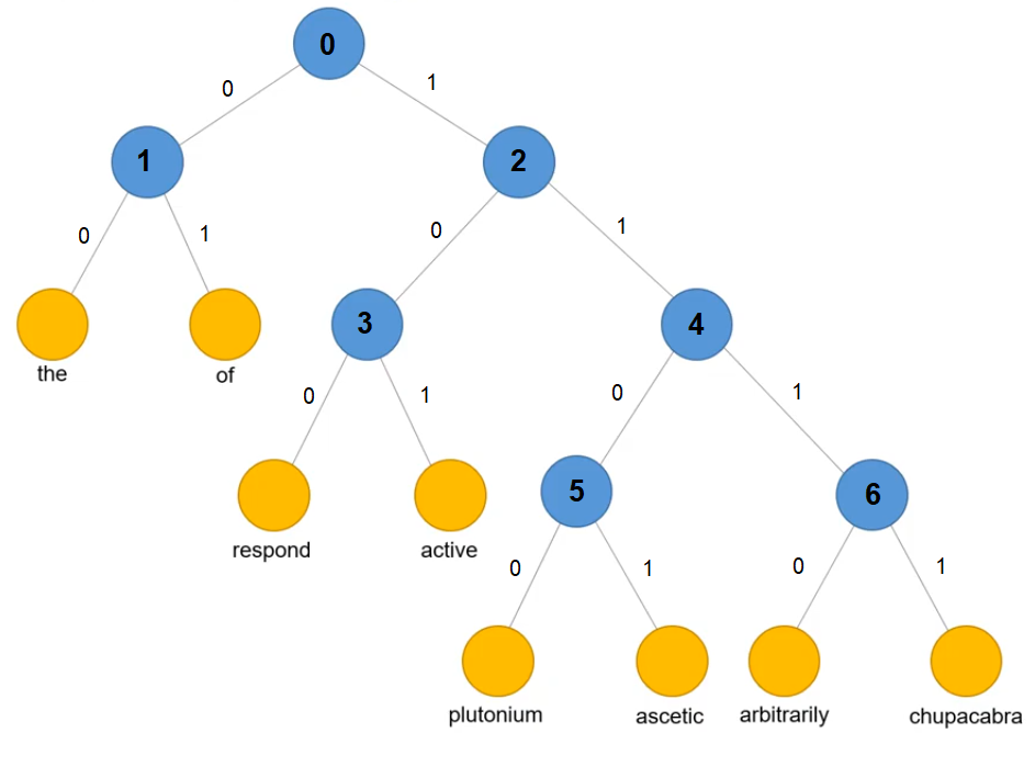
It is a full binary tree with the following characteristics:
- Every internal node has exactly two branches of child node. The internal nodes are depicted with blue circles.
- The leaf node is the vocabulary word, depicted with orange circles.
- The number of internal node is always one less than the number of leaf node.
- The leaf nodes are ordered such that frequent words are located near the root node.
The approximated value will be less accurate, but the computational cost is more efficient. It reduces the complexity from $O(V)$ to $O(log_2{V})$.
aaaabbbbcccdddefgh to get a similar structure as the picture above.
How does the training works?
The input matrix is still the same as a regular Word2Vec architecture. The main difference is on the output matrix. We treat each internal node as a column in the output matrix. Hence, the size of output matrix will be $N \times (V-1)$.
Suppose using the above huffman tree, we train a Skip-gram using the sample (chupacabra, active).
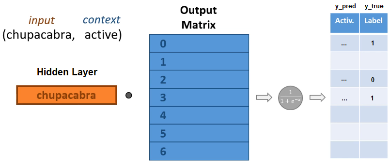
The steps are:
- Take the $N$-dimensional vector of hidden layer of the word
chupacabra. - Travel along the huffman tree to locate the word
active. - For each traversed node:
- Compute the logit score, which is the dot product of the word vector with the corresponding column of output matrix.
- Apply sigmoid activation function to get a probability. We treat this as $\hat{y}$.
- The traversed branch/edge is treated as $y$.
- Compute error and backpropagate, just like the original architecture.
Hyperparameter Tuning
The hyperparameter choice is crucial for model performance, both speed and accuracy. However it varies for different applications. According to this Google Code Archive, the main choices to make are:
-
Architecture:
- Skip-gram: better for rare words and small training set but slower
- CBOW: faster but bias toward frequent words
-
Window size:
- Skip-gram usually around 10
- CBOW around 5
-
Word vectors dimensionality: usually more is better, but not always
-
Training optimization:
- Hierarchical softmax: better for infrequent words
- Negative sampling: better for frequent words, better with low dimensional vectors
-
Sub-sampling frequent words: improve both accuracy and speed for large data sets (useful values are in range 0.1% to 0.001%)
Developed by Samuel Chan and me, Elang is an acronym that combines the phrases Embedding (E) and Language (Lang) Models. Its goal is to help NLP (natural language processing) researchers, Word2Vec practitioners, educators and data scientists be more productive in training language models and explaining key concepts in word embeddings.
from elang.word2vec.builder import build_from_wikipedia

build_from_wikipedia(
    slug="Animal",  # scrape with query
    levels=1,  # levels of articles
    lang="en",  # english language
    model=False,  # don't create model
    save=True)  # save to txt file
wiki_file = open("/content/corpus/txt/wikipedia_branch_Animal_1.txt", "r")
wiki_text = wiki_file.readlines()
Demonstrate what each function does with a sample sentence:
example_sentence = "I'll arrive at the café around 9 PM. See you there! :)"
print(example_sentence)

# contractions.fix()
import contractions
sent = contractions.fix(example_sentence)
print(sent)

# simple_preprocess()
from gensim.utils import simple_preprocess
sent_list = simple_preprocess(sent, deacc = True) # list of tokens
print(' '.join(sent_list))

# optional: Remove stopwords (with the help of nltk)
from nltk.corpus import stopwords
stopword_list = stopwords.words("english")
clean_sent_list = [word for word in sent_list if word not in stopword_list]
print(' '.join(clean_sent_list))
Let's clean our wiki_text (list of sentences) without removing the stopwords.
clean_wiki_text = list(map(contractions.fix, tqdm(wiki_text)))
# clean_wiki_text = list(map(simple_preprocess, clean_wiki_text)) # with no additional parameter
clean_wiki_text = [simple_preprocess(sentence, deacc = True) for sentence in tqdm(clean_wiki_text)] # with additional parameter
from gensim.models.callbacks import CallbackAny2Vec
from time import time

import logging
logging.basicConfig(format='%(asctime)s : %(levelname)s : %(message)s', level=logging.INFO)

class Callback(CallbackAny2Vec):
    def __init__(self):
        self.epoch = 1

    def on_epoch_end(self, model):
        loss = model.get_latest_training_loss()
        if self.epoch == 1:
            print('Loss after epoch {}: {}'.format(self.epoch, loss))
        else:
            print('Loss after epoch {}: {}'.format(
                self.epoch, loss - self.loss_previous_step))
        self.epoch += 1
        self.loss_previous_step = loss
Separate the training into three distinctive steps:
-
Word2Vec(): Set up the parameters of the model one-by-one and leave the model uninitialized. -
.build_vocab(): Builds the vocabulary from a sequence of sentences and thus initialized the model. -
.train(): Finally, trains the model. The loggings here are mainly useful for monitoring, making sure that no threads are executed instantaneously.
from gensim.models import Word2Vec

model = Word2Vec(
    size=300,  # dimensionality of the word vectors
    window=5,  # max distance between context and target word
    min_count=10,  # frequency cut-off
    sg=1,  # skip-gram = 1, CBOW = 0
    cbow_mean=0,  # only applies to CBOW. Use 0 for sum, or 1 for mean of the word vectors
    hs=1,  # using hierarchical softmax
    negative=20,  # negative sampling will not be used, since hs is activated
    ns_exponent=0.75,  # reshape the noise distribution of negative sampling (p)
    alpha=0.005,  # backpropagation learning rate
    seed=123,  # reproducibility
    workers=1)

print(model)
logging.disable(logging.NOTSET)  # enable logging
t = time()

model.build_vocab(clean_wiki_text, progress_per=100)

print('Time to build vocab: {} seconds'.format(round((time() - t), 2)))
logging.disable(logging.INFO)  # disable logging
callback = Callback()  # instead, print out loss for each epoch
t = time()

model.train(clean_wiki_text,
            total_examples=model.corpus_count,  # count of sentences
            epochs=10,  # number of iterations over the corpus,
            compute_loss=True,  # to track model loss
            callbacks=[callback])

print('Time to train the model: {} seconds'.format(round((time() - t), 2)))
print(model)
We can save the trained model using .save() method
Load the pre-trained model using .load() method. I trained the model using wikipedia_branch_Animal_3.txt for a good 1.5 - 2 hours.
from gensim.models import Word2Vec
model = Word2Vec.load("wiki_Animal.model")
print(model)
Step 4. Visualize
The visualization can be useful to understand how Word2Vec works and how to interpret relations between vectors captured from your texts before using them in other machine learning algorithms. By using elang, dimensionality reduction is performed on each word vectors in order to create the two-dimensional plot.
from elang.plot.utils import plot2d, plotNeighbours
plot2d(model, method="TSNE", random_state=123)

similar_w = [w[0] for w in model.wv.most_similar("mouth", topn=20)]
plot2d(model, targets=similar_w, method="TSNE", random_state=123)

Words that have similar meaning (by cosine similarity) tend to plotted next to each other. Therefore, creating a word clusters.
plotNeighbours(model, words=["cat", "strawberry", "indonesia", "blue", "mathematics", "school"],
               method="TSNE", k=10,
               random_state=123, draggable=True)

From the word embedding visualization above, we can conclude 6 clusters as below:
| WORD | COLOR | CATEGORY |
|---|---|---|
| cat | red | animal |
| strawberry | blue | fruit/plant |
| indonesia | violet | country |
| blue | yellow | color |
| mathematics | pink | field of study |
| school | light blue | academic-related |
VOCABULARY LIST
The list of vocabulary is saved on model.wv.vocab
list(model.wv.vocab)[:10]
WORD VECTORS
Check the dimensionality and content of a word vector.
vec = model.wv["dog"]
len(vec)
MOST SIMILAR WORDS
List out topn similar words based on Cosine Similarity.
model.wv.most_similar("dog", topn=5)
OUT-OF-LIST WORD
From a list of words, word vectors can choose one word that has different context among the rest.
model.wv.doesnt_match(['dog', 'cat', 'wolf', 'human', 'eagle'])
model.wv.doesnt_match(['orange', 'red', 'banana', 'blue', 'white'])
WORD RELATIONSHIP
The word vectors can capture word relationship for example:
apple - red = ... - yellowA proper word for this is a fruit with a yellow color.
model.wv.most_similar(positive=['apple', 'yellow'], negative=['red'])
1. Music Recommender at Spotify and Anghami
A user’s listening queue can be used to learn song vectors in the same way that a string of words in text is used to learn word vectors. The assumption is that users will tend to listen to similar tracks in sequence. How these song vectors are then used? One use is to create a kind of music taste vector for a user by averaging together the vectors for songs that a user likes to listen to. This taste vector can then become the query for a similarity search to find songs which are similar to the user’s taste vector.

2. Listing Recommendations at Airbnb
Imagine you are looking for an apartment to rent for your vacation to Paris. As you browse through the available homes, it’s likely that you will investigate a number of listings which fit your preferences and are comparable in features like amenities and design taste. Here the user activity data takes the form of click data, specifically the sequence of listings that a user viewed. Airbnb is able to learn vector representations of their listings by applying the word2vec approach to this data.
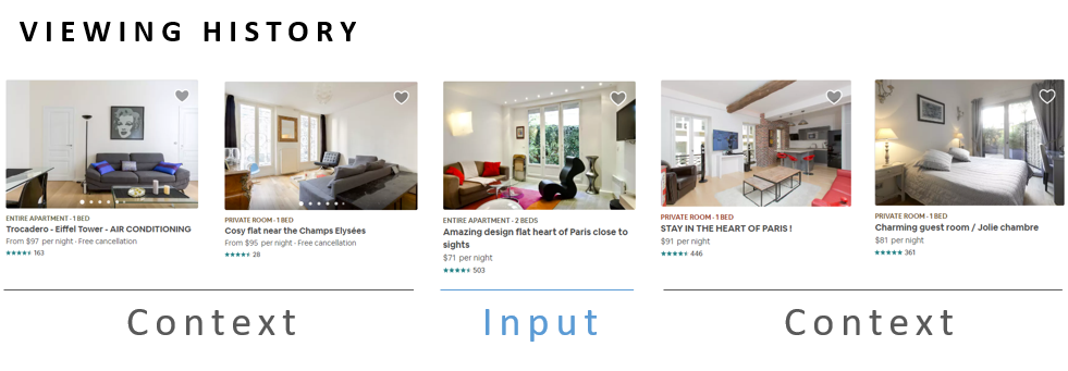
An important piece of the word2vec training algorithm is that for each word that we train on, we select a random handful of words (which are not in the context of that word) to use as negative samples. Airbnb found that in order to learn vectors which could distinguish listings within Paris (and not just distinguish Paris listings from New York listings), it was important that the negative samples be drawn from within Paris.
Their solution to the cold start problem is to simply averaged the vectors of the geographically closest three listings to the new listing to create an initial vector.
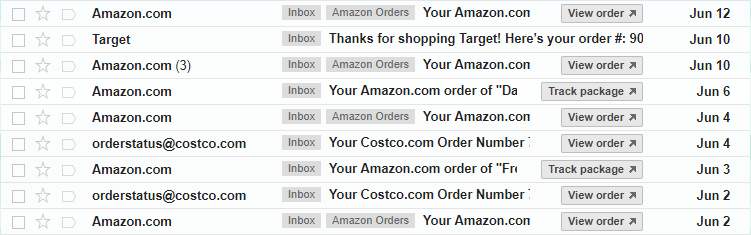
3. Product Recommendations in Yahoo Mail
Yahoo use purchase receipts in a user’s email inbox to form a purchase activity, allowing them in turn to learn product feature vectors which can be used to make product recommendations.
Since online shoppers receive e-mail receipts for their purchases, mail clients are in a unique position to see user purchasing activity across many different e-commerce sites. Even without this advantage, though, Yahoo’s approach seems applicable and potentially valuable to online retailers as well.
Yahoo augmented the word2vec approach with a few notable innovations. The most interesting to me was their use of clustering to promote diversity in their recommendations. After learning vectors for all the products in their database, they clustered these vectors into groups. When making recommendations for a user based on a product the user just purchased, they don’t recommend products from within the same cluster. Instead, they identify which other clusters users most often purchase from after purchasing from the current cluster, and they recommend products from those other clusters instead.
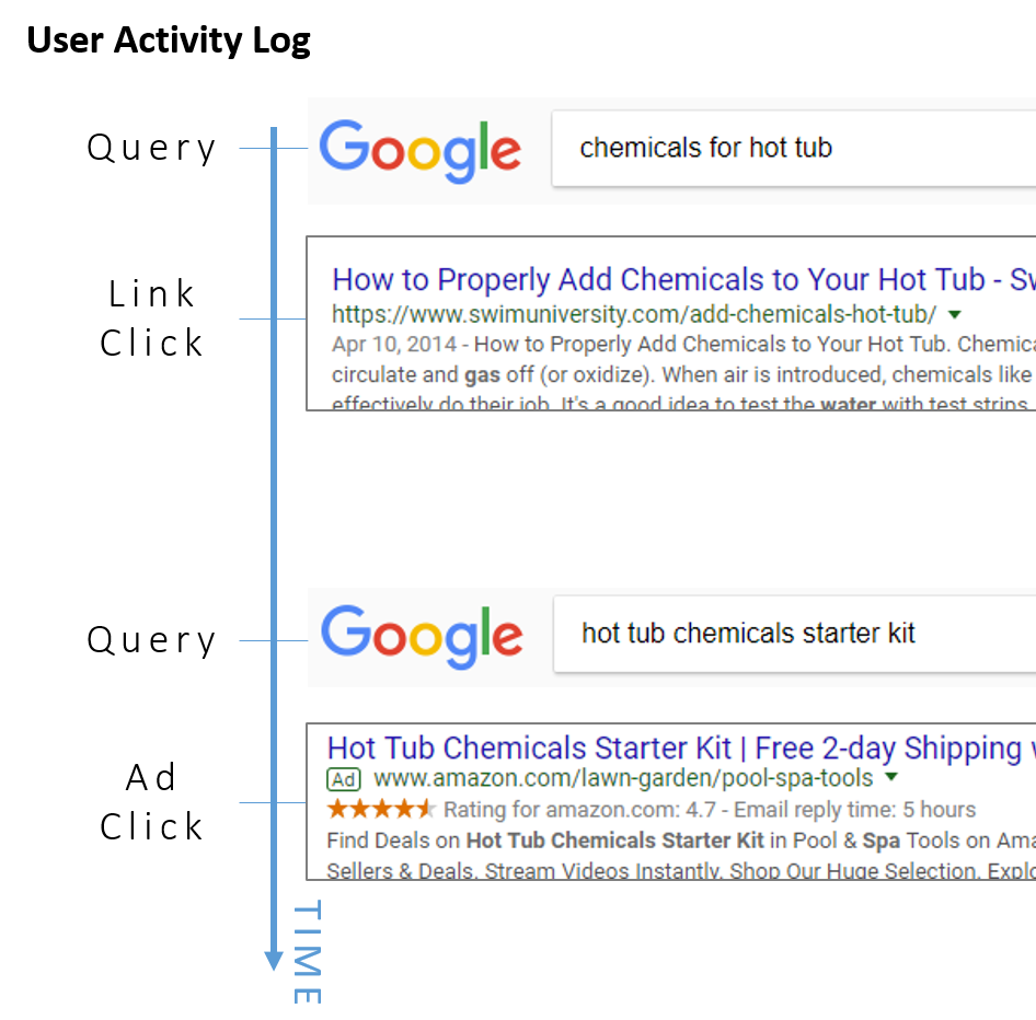
4. Matching Ads to Search Queries on Yahoo Search
The goal is to learn vector representations for search queries and for advertisements in the same embedding space, so that a given search query can be matched against available advertisements in order to find the most relevant ads to show the user.
The training data consists of user search sessions which consist of search queries entered, advertisements clicked, and search result links clicked. The sequence of these user actions is treated like the words in a sentence, and vectors are learned for each of them based on their context–the actions that tend to occur around them. If users often click a particular ad after entering a particular query, then we’ll learn similar vectors for the ad and the query. All three types of actions (searches entered, ads clicked, links clicked) are part of a single “vocabulary” for the model, such that the model doesn’t really distinguish these from one another.
Extension to Word2Vec
Doc2Vec
Doc2Vec is an extension of Word2vec that encodes entire documents as opposed to individual words. Doc2Vec vectors represent the theme or overall meaning of a document. In this case, a document is a sentence, a paragraph, an article or an essay etc. Similar to Word2vec, there are two primary training methods: Distributed Memory Model Of Paragraph Vectors (PV-DM) and Paragraph Vector With A Distributed Bag Of Words (PVDBOW).
Dna2Vec
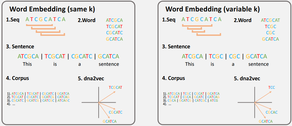
Dna2Vec is a consistent vector representations of variable-length k-mers. The analogies between natural language and DNA are as follow:
- K-mer as the Words
- DNA fragments as the Sentences
- Part/whole of genome as the Corpus
FastText
FastText is proposed by Facebook in 2016. Instead of feeding individual words into the Neural Network, FastText breaks words into several n-grams (sub-words). For instance, the tri-grams for the word apple is app, ppl, and ple. The word embedding vector for apple will be the sum of all these n-grams. After training the Neural Network, we will have word embeddings for all the n-grams given the training dataset.
Rare words can now be properly represented since it is highly likely that some of their n-grams also appears in other words. Even though a word does not exist in the training dataset, the model still capable of figuring out this word is closely related to similar terms.
General Word2Vec Concept
This section will assess your understanding of general Word2Vec and Training Optimization concept.
-
The following three statements are about Word2Vec, choose the CORRECT statement(s):
(i) Word2Vec is an unsupervised learning, even though we use a neural network to train the data.
(ii) In Skip-Gram architecture, the values that are projected onto the hidden layer is the word vector for a certain word in vocabulary.
(iii) In CBOW architecture, the values that are projected onto the hidden layer is the word vector for a certain word in vocabulary.
- a. (i) and (ii)
- b. (i) and (iii)
- c. (ii) and (iii)
- d. all of the above
- e. none of the above
-
Regardless of the Word2Vec architecture, how many training examples will be generated from the sentence "roses are red violets are blue" if the window size is 3?
- a. 18
- b. 21
- c. 24
- d. 27
-
Suppose we have a vocabulary of 5,000 words and learning 100-dimensional Word2Vec embeddings. There will be 500,000 weights of the output matrix to be updated during backpropagation if we don't use a training optimization. Which one of the following statements is CORRECT?
- a. There are also 500,000 weights of the input matrix to be updated during backpropagation.
- b. Using
negative = 20or K = 20 means that only 20 weights (instead of 500,000) of the output matrix will be updated on each batch. - c. Using
ns_exponent = 0or p = 0 means that every single word has a probability of 0.0002 to be choosen as negative sample. - d. Using hierarchical softmax, the size of our output matrix is still 100 x 5,000.
Training Word2Vec
This section will assess your understanding of training Word2Vec using gensim package.
-
Choose one parameter that will speed up the training process if we increase its value, assuming the other parameters remain unchanged.
- a.
min_count - b.
negative - c.
size - d.
window
- a.
-
The following statements are all correct in the process of building a Word2Vec model using
gensim, EXCEPT ...- a. Stemming is rarely performed because a word can lose its semantic meaning.
- b. The training process is separated into three steps for clarity and monitoring.
- c. We doesn't have to set up anything for printing out a training report.
- d. The training sentence is in the form of a "list of lists of tokens".
References
-
Word Embedding and Word2Vec
- Towards Data Science: Introduction to Word Embedding and Word2Vec
- Python Notebook: Understanding Word Vectors
- Machine Learning Plus: Cosine Similarity
- Towards Data Science: NLP 101 Word2Vec Skip-gram and CBOW
- Medium: Word Embedding
- mc.ai: Understand the Softmax Function in Minutes
- Youtube: Hierarchical Softmax in Word2vec
-
Recommender System
-
Potential Uses
- Chris McCormick: Applying Word2vec to Recommenders and Advertising
- mc.ai: An Intuitive Introduction Of Document Vector (Doc2Vec)
- arXiv Paper: dna2vec
- Data Science Hongkong: Application of Word2Vec to Represent Biological Sequences
- Towards Data Science: Word2Vec and FastText Word Embedding with Gensim