Breast Cancer Wisconsin Classification
A simple machine learning workflow to classify whether a mass is classified as malignant or benign cancer, based on the clinical measurement of cell nucleus. Four models are compared to achieve best F1 score: logistic regression, support vector, decision tree, and random forest classifier. Each models are tuned using grid search cross-validation and threshold tuning. This post is dedicated for a final project of Indonesia AI Mentorship - Machine Learning Program.

- Load Libraries
- Data Loading
- Data Visualization
- Distribution
- Data Preprocessing
- Data Modeling
- Conclusion
import pandas as pd
import numpy as np

# data visualization
import matplotlib.pyplot as plt
import seaborn as sns
import graphviz

# modeling
from sklearn.preprocessing import LabelEncoder
from sklearn.model_selection import train_test_split
from sklearn.linear_model import LogisticRegression
from sklearn.svm import SVC
from sklearn.tree import DecisionTreeClassifier, export_graphviz
from sklearn.ensemble import RandomForestClassifier
from sklearn.metrics import recall_score, precision_score, f1_score, classification_report
from sklearn.model_selection import GridSearchCV

# other
from IPython.display import display, Math, HTML

# setting
plt.style.use('seaborn')
pd.set_option('display.float_format', lambda x: '%.5f' % x)
pd.set_option('display.max_colwidth', None)
pd.options.plotting.backend = "plotly"
Data Loading
The cancer dataset used is provided from Kaggle.
cancer = pd.read_csv("data_input/data.csv")
cancer.info()
There are 569 observations and 33 columns with the following description:
-
id: ID number -
diagnosis: M = Malignant, B = Benign (target variable)
Ten real-valued features are computed for each cell nucleus:
-
radius: mean of distances from center to points on the perimeter -
texture: standard deviation of gray-scale values perimeterarea-
smoothness: local variation in radius lengths -
compactness: perimeter^2 / area - 1.0 -
concavity: severity of concave portions of the contour -
concave points: number of concave portions of the contour symmetry-
fractal dimension: "coastline approximation" - 1
The feature above is calculated based on their mean, se (standard error), and worst (largest).
missing = cancer.isnull().sum()
missing[missing>0]
We can remove the id column because it is not used as a feature, and the Unnamed: 32 column because it is an empty column.
cancer.drop(['id', 'Unnamed: 32'], axis=1, inplace=True)
sns.countplot(x='diagnosis', data=cancer);

plt.figure(figsize=(15, 15))
sns.heatmap(cancer.corr(), annot=True, linewidths=0.5, fmt='.2f');

cancer_longer = cancer.melt(id_vars='diagnosis', var_name='features')
g = sns.FacetGrid(data=cancer_longer, col='features',
                  col_wrap=10, sharey=False)
g.map_dataframe(sns.boxplot, x='diagnosis', y='value', hue='diagnosis')
g.add_legend()
plt.show()

median = cancer_longer.groupby(['diagnosis', 'features']).quantile(0.5)['value'].unstack(level='diagnosis')
median['Median Difference'] = median['M'] - median['B']
median = median.sort_values('Median Difference')
pd.concat([median.head(3), median.tail(3)])
The table above shows the median value of each features for Benign and Malignant cancer. The median difference is calculated by subtracting median of Benign from Malignant. In general, the median value for majority of the features is greater for Malignant than Benign except for texture_se, symmetry_se, and smoothness_se. The most obvious feature is area, because the median value of Malignant is more than twice the median value of Benign.
We have to encode the target variable diagnosis using LabelEncoder. Encoding is not needed for the features since all value are numeric.
X = cancer.drop(columns=['diagnosis'])

le = LabelEncoder()
y = le.fit_transform(cancer['diagnosis'])
le_name_mapping = dict(zip(le.classes_, le.transform(le.classes_)))
le_name_mapping
LabelEncoder, the target value Benign is mapped into 0, while Malignant is mapped into 1
Train-test splitting with 75:25 proportion.
X_train, X_test, y_train, y_test = train_test_split(X, y, test_size=0.25, random_state=0)
print(f"X_train shape: {X_train.shape}")
print(f"X_test shape: {X_test.shape}")
print(f"y_train shape: {y_train.shape}")
print(f"y_test shape: {y_test.shape}")
Data Modeling
We are going to compare four binary classification models: logistic regression, support vector, decision tree, and random forest classfier. The positive target class is Malignant (1), while the negative is Benign (0).
We are going to consider the following evaluation metrics:
- Recall: what percentage of patients with Malignant can the model detect?
- Precision: of the patients predicted to be Malignant, what percentage were truly Malignant?
- F1 score: weighted average of Recall and Precision.
$F1 = 2 \times \frac{Recall \times Precision}{Recall+Precision}$
Types of errors:
- False Positive: Patients who actually have benign cancer (Benign), predicted by the model as Malignant. This can cause panic in the patient, but the patient will receive further consultation or treatment as a preventive measure, so that patient safety is guaranteed.
- False Negative: Patients who actually have malignant cancer (Malignant), predicted by the model to be Benign. This can jeopardize the patients' safety because they are not taken seriously.
logreg = LogisticRegression(max_iter=np.inf, random_state=123)
logreg.fit(X_train, y_train)
We define a function threshold_tuning to further tune the threshold to get the largest F1 score.
def threshold_tuning(model, X, y):
    y_pred_prob = model.predict_proba(X)[:, 1]  # probability

    eval_list = []
    for threshold in np.linspace(0, 0.99, 100):
        y_pred = (y_pred_prob > threshold).astype(int)  # threshold cut-off

        # evaluation metric
        eval_dict = {
            'Threshold': threshold,
            'Recall': recall_score(y, y_pred),
            'Precision': precision_score(y, y_pred),
            'F1': f1_score(y, y_pred)
        }

        eval_list.append(eval_dict)

    # tuning result
    eval_df = pd.DataFrame(eval_list).set_index('Threshold')
    eval_df.columns = eval_df.columns.set_names('Metrics')
    max_f1 = eval_df.sort_values('F1', ascending=False).head(1)
    optimal_threshold = max_f1.index.values[0]

    # plotting
    fig = eval_df.plot(title="Threshold Tuning")
    fig.add_shape(dict(type="line",
                       x0=optimal_threshold, y0=0,
                       x1=optimal_threshold, y1=1))

    # print classification report using max F1
    y_pred_optimal = (y_pred_prob > optimal_threshold).astype(int)
    print(classification_report(y, y_pred_optimal,
          target_names=['Benign', 'Malignant']))

    return eval_df.sort_values('F1', ascending=False), fig
logreg_tuning, fig = threshold_tuning(logreg, X_test, y_test)
HTML(fig.to_html(include_plotlyjs='cdn'))
For logistic regression, we use threshold = 0.84 to get the largest F1 score on the testing set. Next, we would like to interpret the model via estimate (intercept and coefficient). The following predictors have been sorted by coefficient from largest to smallest:
logreg_interpret = pd.DataFrame(np.append(logreg.intercept_, logreg.coef_), columns=['Estimate (Logit)'])
logreg_interpret.index = ['intercept'] + list(X.columns)
logreg_interpret['Odds Ratio'] = logreg_interpret['Estimate (Logit)'].transform(np.exp)
logreg_interpret.sort_values('Estimate (Logit)', ascending=False)
Examples:
- An increase of 1 unit of
concativity_worstwill increase the possibility of a cancer to be malignant by 194.308% (its Odds Ratio - 1) - An increase of 1 unit of
texture_sewill reduce the possibility of a cancer to be malignant by 62.584% (1 - its Odds Ratio)
svc_parameters = {
    'kernel': ['linear', 'poly', 'rbf', 'sigmoid'],
    'C': [0.1, 1, 10]
}
svc = SVC(random_state=123)
svc_grid = GridSearchCV(svc, svc_parameters, cv=3, scoring='f1')
svc_grid.fit(X_train, y_train)
pd.DataFrame(svc_grid.cv_results_).sort_values('rank_test_score').head(3)[['rank_test_score', 'params', 'mean_test_score', 'std_test_score']]
Re-training the support vector model with a combination of parameters that produces the largest F1.
svc_grid directly to predict a class, but in this case we would like to predict a probability to tune the threshold. It will take a long time if we use probability=True during the grid search because for all combinations of parameters the probability will be calculated. What we really want is the probability only for the best combination of parameters.
svc_best = SVC(**svc_grid.best_params_, probability=True, random_state=123)
svc_best.fit(X_train, y_train)
We further tune the support vector model using defined threshold_tuning function.
svc_tuning, fig = threshold_tuning(svc_best, X_test, y_test)
HTML(fig.to_html(include_plotlyjs='cdn'))
For support vector, we use threshold = 0.42 to get the largest F1 score on the testing set.
dtc_parameters = {
    'criterion': ['gini', 'entropy'],
    'splitter': ['best', 'random'],
    'max_features': [2, 'sqrt', 'log2'],
    'min_samples_leaf': range(1, 10, 2)
}
dtc = DecisionTreeClassifier(random_state=123)
dtc_grid = GridSearchCV(dtc, dtc_parameters, cv=3, scoring='f1')
dtc_grid.fit(X_train, y_train)
pd.DataFrame(dtc_grid.cv_results_).sort_values('rank_test_score').head(3)[['rank_test_score', 'params', 'mean_test_score', 'std_test_score']]
We further tune the decision tree model using defined threshold_tuning function. We don't need to re-train the best model as in the previous support vector section, because dtc_grid can be directly used to predict probability.
dtc_tuning, fig = threshold_tuning(dtc_grid, X_test, y_test)
HTML(fig.to_html(include_plotlyjs='cdn'))
For decision tree, we use threshold = 0.5 to get the largest F1 score on the testing set. Next, we would like to interpret the model visually.
dot_data = export_graphviz(
    dtc_grid.best_estimator_,
    feature_names=X.columns,
    class_names=['Benign', 'Malignant'],
    impurity=False,
    leaves_parallel=True,
    filled=True,
    rounded=True)
graph = graphviz.Source(dot_data)
# display(graph)
graph.format = "png"
graph.render("assets/2020-10-26-breast-cancer-wisconsin-classification/decision_tree_breast_cancer");
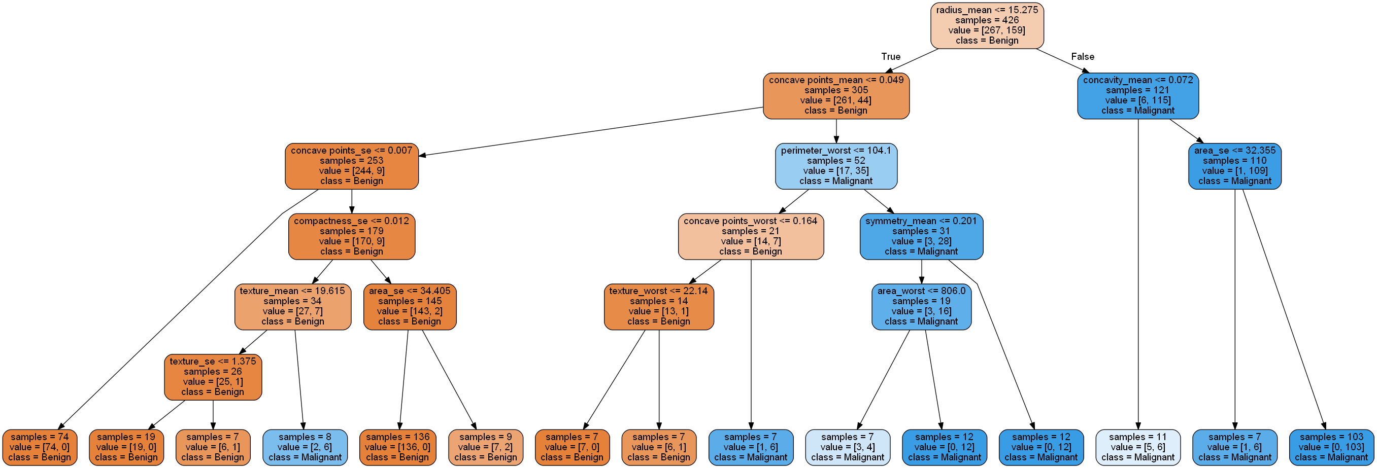
The decision tree can be traversed from the root (top) to leaf (bottom). The predicted class is labeled for each leaf. Each node will be separated by a condition, if True then traverse to the left, otherwise to the right.
rfc_parameters = {
    'n_estimators': [100, 200, 300],
    'criterion': ['gini', 'entropy'],
    'max_features': [2, 'sqrt', 'log2']
}
rfc = RandomForestClassifier(random_state=123)
rfc_grid = GridSearchCV(rfc, rfc_parameters, cv=3, scoring='f1')
rfc_grid.fit(X_train, y_train)
pd.DataFrame(rfc_grid.cv_results_).sort_values('rank_test_score').head(3)[['rank_test_score', 'params', 'mean_test_score', 'std_test_score']]
We further tune the random forest model using defined threshold_tuning function. We don't need to re-train the best model as in the previous support vector section, because rfc_grid can be directly used to predict probability.
rfc_tuning, fig = threshold_tuning(rfc_grid, X_test, y_test)
HTML(fig.to_html(include_plotlyjs='cdn'))
For random forest, we use threshold = 0.46 to get the largest F1 score on the testing set. Next, we would like to interpret the model based on feature importances. Here are the top 10 features that are most important in classifying whether a cancer is benign or malignant:
pd.options.plotting.backend = "matplotlib"

var_imp = pd.DataFrame({
    'Feature': X.columns,
    'Importance': rfc_grid.best_estimator_.feature_importances_
}).set_index('Feature')

var_imp.sort_values('Importance', ascending=False).head(10).sort_values(
    'Importance').plot.barh(title='Top 10 Feature Importances');

final_result = pd.concat([
    logreg_tuning.head(1),
    svc_tuning.head(1),
    dtc_tuning.head(1),
    rfc_tuning.head(1)]).reset_index()
final_result.index = ['Logistic Regression', 'Support Vector Classifier',
                      'Decision Tree Classifier', 'Random Forest Classifier']
final_result
Each model has its advantages and disadvantages as shown in the image below:
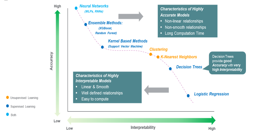
If we have to choose between the four models, we prefer the model that results in high performance in classifying cancer since the safety and life of a patient are crucial in the medical field. Thus, we choose Random Forest Classifier with a threshold of 0.46 because it has the highest F1 score, and the importance of each feature can be measured using Feature Importances (although the influence of positive or negative directions is unknown as in Logistic Regression).