MNIST Digit Classifier using PyTorch
A simple workflow on how to build a multilayer perceptron to classify MNIST handwritten digits using PyTorch. We define a custom Dataset class to load and preprocess the input data. The neural network architecture is built using a sequential layer, just like the Keras framework. We define the training and testing loop manually using Python for-loop. The final model is evaluated using a standard accuracy measure.

- Background
- Installation
- Libraries
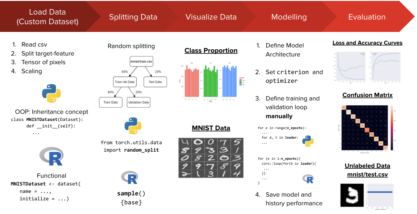
- Workflow
- Load Data
- Visualize Data
- Define Model Architecture
- Train the Model
- Test the Model
- Predict the Unlabeled Data
- References
- Further Readings
Deep learning is part of a broader family of machine learning methods based on artificial neural networks with representation learning. These neural networks attempt to simulate the behavior of the human brain allowing it to “learn” from large amounts of data. Not only possible to apply in large amounts of data, but it also allows to deal with unstructured data such as image, text, and sound.
You can try to implement a neural network from scratch. But, do you think this is a good idea when building deep learning models on a real-world dataset? It is definitely possible if you have days or weeks to spare waiting for the model to build. But, in any conditions we have many constrain to do it e.g time and cost.
Here is the good news, now we can use deep learning frameworks that aim to simplify the implementation of complex deep learning models. Using these frameworks, we can implement complex models like convolutional neural networks in no time.
A deep learning framework is a tool that allows us to build deep learning models more easily and quickly. They provide a clear and concise way for defining models using a collection of pre-built and optimized components. Instead of writing hundreds of lines of code, we can use a suitable framework to help us to build such a model quickly.

| Keras | PyTorch |
|---|---|
| Keras was released in March 2015 | While PyTorch was released in October 2016 |
| Keras has a high level API | While PyTorch has a low level API |
| Keras is comparatively slower in speed | While PyTorch has a higher speed than Keras, suitable for high performance |
| Keras has a simple architecture, making it more readable and easy to use | While PyTorch has very low readablility due to a complex architecture |
| Keras has a smaller community support | While PyTorch has a stronger community support |
| Keras is mostly used for small datasets due to its slow speed | While PyTorch is preferred for large datasets and high performance |
| Debugging in Keras is difficult due to presence of computational junk | While debugging in PyTorch is easier and faster |
| Keras provides static computation graphs | While PyTorch provides dynamic computation graphs |
| Backend for Keras include:TensorFlow, Theano and Microsoft CNTK backend | While PyTorch has no backend implementation |
Please ensure you have installed the following packages to run sample notebook. Here is the short instruction on how to create a new conda environment with those package inside it.
- Open the terminal or Anaconda command prompt.
-
Create new conda environment by running the following command.
conda create -n <env_name> python=3.7 -
Activate the conda environment by running the following command.
conda activate <env_name> -
Install additional packages such as
pandas,numpy,matplotlib,seaborn, andsklearninside the conda environment.pip install pandas numpy matplotlib seaborn scikit-learn -
Install
torchinto the environment.pip3 install torch torchvision torchaudio
After the required package is installed, load the package into your workspace using the import
import pandas as pd  # for read_csv
import numpy as np  # for np.Inf
import matplotlib.pyplot as plt  # visualization
import seaborn as sns  # heatmap visualization
from sklearn.metrics import confusion_matrix, classification_report  # evaluation metrics
import pickle  # serialization

import torch
from torch.utils.data import Dataset, DataLoader, random_split
import torch.nn as nn
import torch.nn.functional as F
import torch.optim as optim

plt.style.use("seaborn")
torch.manual_seed(123)
Let's start implement our existing knowledge of neural network using torch in Python to solve an image classification problem. We'll use famous MNIST Handwritten Digits Data as our training dataset. It consists of 28 by 28 pixels grayscale images of handwritten digits (0 to 9) and labels for each image indicating which digit it represents. There are two files of data to be downloaded: train.csv is pixel data with actual digit label, whereas test.csv is pixel data without the actual digit label. Here are some sample image from dataset:
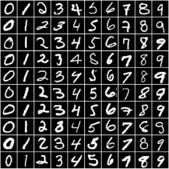
It's evident that these images are relatively small in size, and recognizing the digits can sometimes be challenging even for the human eye. While it's useful to look at these images, there's just one problem here: PyTorch doesn't know how to work with images. We need to convert the images into tensors. We can do this by specifying a transform while creating our dataset.
PyTorch Dataset allow us to specify one or more transformation functions that are applied to the images as they are loaded. We'll use the torch.tensor() to convert the pixel values into tensors.
class MNISTDataset(Dataset):
    # constructor
    def __init__(self, file_path):
        # read data
        df = pd.read_csv(file_path)

        target_col = "label"
        self.label_exist = target_col in df.columns

        if self.label_exist:
            # split feature-target
            X = df.drop(columns=target_col).values
            y = df[target_col].values

            # convert numpy array to tensor
            self.y = torch.tensor(y)
        else:
            X = df.values

        self.X = torch.tensor(X, dtype=torch.float32)

        # scaling
        self.X /= 255

    # for iteration
    def __getitem__(self, idx):
        if self.label_exist:
            return self.X[idx], self.y[idx]
        else:
            return self.X[idx]

    # to check num of observations
    def __len__(self):
        return self.X.size()[0]
mnist_data = MNISTDataset("data_input/mnist/train.csv")
print(mnist_data.X.size())
SPLIT_PROP = 0.8
BATCH_SIZE = 16
While building real-world machine learning models, it is quite common to split the dataset into three parts:
- Training set - used to train the model, i.e., compute the loss and adjust the model's weights using gradient descent.
- Validation set - used to evaluate the model during training, adjust hyperparameters (learning rate, etc.), and pick the best version of the model.
- Test set - used to compare different models or approaches and report the model's final accuracy.
In the MNIST dataset, there are 42,000 images in train.csv and 784 images in test.csv. The test set is standardized so that different researchers can report their models' results against the same collection of images.
Since there's no predefined validation set, we must manually split the 42,000 images into training, validation, and test datasets. Let's set aside 42,000 randomly chosen images for validation. We can do this using the random_split method from torch.
train_val_size = int(SPLIT_PROP * len(mnist_data))
test_size = len(mnist_data) - train_val_size

train_size = int(SPLIT_PROP * train_val_size)
val_size = train_val_size - train_size

# train-val-test split
train_mnist, val_mnist, test_mnist = random_split(mnist_data, [train_size, val_size, test_size])

print(f"Training set: {len(train_mnist):,} images")
print(f"Validation set: {len(val_mnist):,} images")
print(f"Testing set: {len(test_mnist):,} images")
It's essential to choose a random sample for creating a validation and test set. Training data is often sorted by the target labels, i.e., images of 0s, followed by 1s, followed by 2s, etc. If we create a validation set using the last 20% of images, it would only consist of 8s and 9s. In contrast, the training set would contain no 8s or 9s. Such a training-validation would make it impossible to train a useful model.
We can now create DataLoader to help us load the data in batches. We'll use a batch size of 16. We set shuffle=True for the data loader to ensure that the batches generated in each epoch are different. This randomization helps generalize & speed up the training process.
train_loader = DataLoader(train_mnist, batch_size=BATCH_SIZE, shuffle=True)
val_loader = DataLoader(val_mnist, batch_size=BATCH_SIZE, shuffle=True)
test_loader = DataLoader(test_mnist, batch_size=BATCH_SIZE, shuffle=True)

print(f"Training data loader: {len(train_loader):,} images per batch")
print(f"Validation data loader: {len(val_loader):,} images per batch")
print(f"Testing data loader: {len(test_loader):,} images per batch")
Let's check the proportion of each class labels, since it is important to ensure that the model can learn each digit in a balanced and fair manner. We check the distribution of digits in training, validation, and also test set.
# get target variable proportion
train_prop = mnist_data.y[train_mnist.indices].bincount()
val_prop = mnist_data.y[val_mnist.indices].bincount()
test_prop = mnist_data.y[test_mnist.indices].bincount()

# visualization
fig, axes = plt.subplots(1, 3, figsize=(12, 3))
for ax, prop, title, col in zip(axes, [train_prop, val_prop, test_prop], ['Train', 'Validation', 'Test'], 'bgr'):
    class_target = range(0, 10)
    ax.bar(class_target, prop, color=col)
    ax.set_title(title)
    ax.set_xticks(class_target)
    ax.set_xlabel("Label")

axes[0].set_ylabel("Frequency")
plt.show()

The distribution of our class labels do seem to be spread out quite evenly, so there's no problem. Next, we visualize a couple of images from train_loader:
class_label = ['zero', 'one', 'two', 'three',
               'four', 'five', 'six', 'seven', 'eight', 'nine']

images, labels = next(iter(train_loader))
images = images.reshape((train_loader.batch_size, 28, 28))

fig, axes = plt.subplots(2, 8, figsize=(12, 4))
for ax, img, label in zip(axes.flat, images, labels):
    ax.imshow(img, cmap="gray")
    ax.axis("off")
    ax.set_title(class_label[label])
plt.tight_layout()

We'll create a neural network with three layers: two hidden and one output layer. Additionally, we'll use ReLu activation function between each layer. Let's create a nn.Sequential object, which consists of linear fully-connected layer:
- The input size is 784 nodes as the MNIST dataset consists of 28 by 28 pixels
- The hidden sizes are 128 and 64 respectively, this number can be increased or decreased to change the learning capacity of the model
- The output size is 10 as the MNIST dataset has 10 target classes (0 to 9)
input_size = 784
hidden_sizes = [128, 64]
output_size = 10

model = nn.Sequential(
    nn.Linear(input_size, hidden_sizes[0]),
    nn.ReLU(),
    nn.Linear(hidden_sizes[0], hidden_sizes[1]),
    nn.ReLU(),
    nn.Linear(hidden_sizes[1], output_size)  # logit score
)
model
A little bit about the mathematical detail: The image vector of size 784 are transformed into intermediate output vector of length 128 then 64 by performing a matrix multiplication of inputs matrix. Thus, input and layer1 outputs have linear relationship, i.e., each element of layer outputs is a weighted sum of elements from inputs. Thus, even as we train the model and modify the weights, layer1 can only capture linear relationships between inputs and outputs.
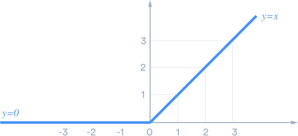
Activation function such as Rectified Linear Unit (ReLU) is used to introduce non-linearity to the model. It has the formula relu(x) = max(0,x) i.e. it simply replaces negative values in a given tensor with the value 0. We refer to ReLU as the activation function, because for each input certain outputs are activated (those with non-zero values) while others turned off (those with zero values). ReLU can be seen visually as follows:
The output layer returns a batch of vectors of size 10. This predicted output is then being compared with actual label, quantified by using nn.CrossEntropyLoss(). It combines LogSoftmax and NLLLoss (Negative Log Likelihood Loss) in one single class.
The loss value is used to update the parameter weights in the model. The parameter update algorithm can be implemented via an optimizer. In this case, we are using torch.optim.Adam() with learning rate (lr=0.001).
criterion = nn.CrossEntropyLoss()

# specify optimizer (Adam) and learning rate = 0.001
optimizer = torch.optim.Adam(model.parameters(), lr=0.001)
Using torch, we have to manually loop the data per epoch to train the model. Here are the training loop for one epoch:
- Clear gradients of all optimized variables from
optimizer - Forward pass: compute predicted output by passing input data to the
model - Calculate the loss based on specified
criterion - Backward pass: compute gradient of the loss with respect to
modelparameters - Perform parameter update using
optimizeralgorithm - Accumulate training loss and accuracy
Inside the training loop, we also validate the model by performing the following steps:
- Forward pass: compute predicted output by passing input data to the
model - Calculate the loss based on specified
criterion - Accumulate validation loss and accuracy
Special notes:
- If you use
DropoutorBatchNormlayer, don't forget to usemodel.train()when training the model andmodel.eval()when validating/testing the model so that the layer behaves accordingly. - Don't forget to set
torch.no_grad()before validating the model to disable the gradient calculation since we are not updating the parameters.
But first let's us define evaluate_accuracy to calculate accuracy given the predicted logits and y_true actual label.
def evaluate_accuracy(logits, y_true):
    # get index with the largest logit value PER OBSERVATION
    _, y_pred = torch.max(logits, dim=1)

    # calculate proportion of correct prediction
    correct_pred = (y_pred == y_true).float()
    acc = correct_pred.sum() / len(correct_pred)

    return acc * 100
Define training loop with the following parameters:
-
model: untrained model -
train_loader: data train of aDataLoaderobject -
val_loader: data validation of aDataLoaderobject -
criterion: loss function to be optimized -
optimizer: optimization algorithm to used on themodelparameters -
n_epochs: number of training epochs -
model_file_name: file name of serialized model. During the training loop, model with the lowest validation loss will be saved as a serialized model with.ptextension.
def train(model, train_loader, val_loader, criterion, optimizer, n_epochs, model_file_name='model.pt'):
    # initialize container variable for model performance results per epoch
    history = {
        'n_epochs': n_epochs,
        'loss': {
            'train': [],
            'val': []
        },
        'acc': {
            'train': [],
            'val': []
        }
    }

    # initialize tracker for minimum validation loss
    val_loss_min = np.Inf

    # loop per epoch
    for epoch in range(n_epochs):
        # initialize tracker for training performance
        train_acc = 0
        train_loss = 0

        ###################
        # train the model #
        ###################

        # prepare model for training
        model.train()

        # loop for each batch
        for data, target in train_loader:
            # STEP 1: clear gradients
            optimizer.zero_grad()
            # STEP 2: forward pass
            output = model(data)
            # STEP 3: calculate the loss
            loss = criterion(output, target)
            # STEP 4: backward pass
            loss.backward()
            # STEP 5: perform parameter update
            optimizer.step()
            # STEP 6: accumulate training loss and accuracy
            train_loss += loss.item() * data.size(0)
            acc = evaluate_accuracy(output, target)
            train_acc += acc.item() * data.size(0)

        ######################
        # validate the model #
        ######################

        # disable gradient calculation
        with torch.no_grad():
            # initialize tracker for validation performance
            val_acc = 0
            val_loss = 0

            # prepare model for evaluation
            model.eval()

            # loop for each batch
            for data, target in val_loader:
                # STEP 1: forward pass
                output = model(data)
                # STEP 2: calculate the loss
                loss = criterion(output, target)
                # STEP 3: accumulate validation loss and accuracy
                val_loss += loss.item() * data.size(0)
                acc = evaluate_accuracy(output, target)
                val_acc += acc.item() * data.size(0)

        ####################
        # model evaluation #
        ####################

        # calculate average loss over an epoch
        train_loss /= len(train_loader.sampler)
        val_loss /= len(val_loader.sampler)
        history['loss']['train'].append(train_loss)
        history['loss']['val'].append(val_loss)

        # calculate average accuracy over an epoch
        train_acc /= len(train_loader.sampler)
        val_acc /= len(val_loader.sampler)
        history['acc']['train'].append(train_acc)
        history['acc']['val'].append(val_acc)

        # print training progress per epoch
        print(f'Epoch {epoch+1:03} | Train Loss: {train_loss:.5f} | Val Loss: {val_loss:.5f} | Train Acc: {train_acc:.2f} | Val Acc: {val_acc:.2f}')

        # save model if validation loss has decreased
        if val_loss <= val_loss_min:
            print(
                f'Validation loss decreased ({val_loss_min:.5f} --> {val_loss:.5f})  Saving model to {model_file_name}...')
            torch.save(model.state_dict(), model_file_name)
            val_loss_min = val_loss

        print()

    # return model performance history
    return history
history = train(
    model, train_loader, val_loader, criterion, optimizer, n_epochs=20,
    model_file_name='cache/model-mnist-digit.pt'
)
with open('cache/history-mnist-digit.pickle', 'wb') as f:
    pickle.dump(history, f, protocol=pickle.HIGHEST_PROTOCOL)
Visualize the loss and accuracy from history to see the model performance for each epoch.
# load previously saved history dictionary
with open('cache/history-mnist-digit.pickle', 'rb') as f:
    history = pickle.load(f)

# visualization
epoch_list = range(1, history['n_epochs']+1)

fig, axes = plt.subplots(1, 2, figsize=(18, 6))
for ax, metric in zip(axes, ['loss', 'acc']):
    ax.plot(epoch_list, history[metric]['train'], label=f"train_{metric}")
    ax.plot(epoch_list, history[metric]['val'], label=f"val_{metric}")
    ax.set_xlabel('epoch')
    ax.set_ylabel(metric)
    ax.legend()

From the visualization, we can deduct that the model is a good enough since the difference of model performance on training and validation is not too much different, and the accuracy is converging at 96-97%.
In this section, we are going to test the model performance by using confusion matrix. Here are the steps:
- Forward pass: compute predicted output by passing input data to the trained
model - Get predicted label by retrieve index with the largest logit value per observation
- Append actual and predicted label to
y_testandy_predrespectively
model.load_state_dict(torch.load('cache/model-mnist-digit.pt'))
y_test = []
y_pred = []

# disable gradient calculation
with torch.no_grad():
    # prepare model for evaluation
    model.eval()

    # loop for each data
    for data, target in test_loader:
        # STEP 1: forward pass
        output = model(data)
        # STEP 2: get predicted label
        _, label = torch.max(output, dim=1)
        # STEP 3: append actual and predicted label
        y_test += target.numpy().tolist()
        y_pred += label.numpy().tolist()
Create a confusion matrix heatmap using seaborn and classification report by using sklearn to know the final model performance on test data.
plt.subplots(figsize=(10, 8))
ax = sns.heatmap(confusion_matrix(y_test, y_pred), annot=True, fmt="d")
ax.set_xlabel("Predicted Label")
ax.set_ylabel("Actual Label")
plt.show()

print(classification_report(y_test, y_pred))
Eventually, the model achieves 97% accuracy and other metrics reach >= 92% on unseen data.
In this last section, we use the trained model to predict the unlabeled data from test.csv, which only consists 784 columns of pixel without the actual label.
mnist_data_unlabeled = MNISTDataset("data_input/mnist/test.csv")
unlabeled_loader = DataLoader(mnist_data_unlabeled, batch_size=1, shuffle=True)

print(mnist_data_unlabeled.X.size())
Each image is feeded into the model and F.softmax activation function will be applied on the output value to convert logit scores to probability. The visualization tells us the predicted probability given an image, and then class with the highest probability will be the final predicted label of that image.
for idx in range(3):
    # get image from loader
    image = next(iter(unlabeled_loader))
    image = image.reshape((28, 28))

    ##############
    # prediction #
    ##############

    with torch.no_grad():
        # forward pass
        output = model(image.reshape(1, -1))
        # calculate probability
        prob = F.softmax(output, dim=1)

    #################
    # visualization #
    #################

    fig, axes = plt.subplots(1, 2, figsize=(8, 4))

    # show digit image
    axes[0].imshow(image, cmap="gray")
    axes[0].axis("off")

    # predicted probability barplot
    axes[1].barh(range(0, 10), prob.reshape(-1))
    axes[1].invert_yaxis()
    axes[1].set_yticks(range(0, 10))
    axes[1].set_xlabel("Predicted Probability")

    plt.tight_layout()
    plt.show()


There's a lot of scope to experiment here, and I encourage you to use the interactive nature of Jupyter to play around with the various parameters. Here are a few ideas:
-
Try changing the size of the hidden layer, or add more hidden layers and see if you can achieve a higher accuracy.
-
Try changing the batch size and learning rate to see if you can achieve the same accuracy in fewer epochs.
-
Compare the training times on a CPU vs. GPU. Do you see a significant difference. How does it vary with the size of the dataset and the size of the model (no. of weights and parameters)?
-
Try building a model for a different dataset, such as the CIFAR10 or CIFAR100 datasets.
Here are some references for further reading:
-
A visual proof that neural networks can compute any function, also known as the Universal Approximation Theorem.
-
But what is a neural network? - A visual and intuitive introduction to what neural networks are and what the intermediate layers represent
-
Stanford CS229 Lecture notes on Backpropagation - for a more mathematical treatment of how gradients are calculated and weights are updated for neural networks with multiple layers.