Introduction

The anthropometric analysis of the human face is an important study for performing craniofacial plastic and reconstructive surgeries. Facial anthropometric is affected by various factors such as age, gender, ethnicity, socioeconomic status, environment, and region. Plastic surgeons who repair and reconstruct facial deformities find the anatomical dimensions of the facial structures useful for their surgeries. These dimensions result from the physical or facial appearance of an individual. Factors like culture, personality, ethnic background, age, eye appearance, and symmetry contribute majorly to facial appearance or aesthetics.

Note: The following post is an extension from my notebook submitted to DPhi Challenges

Download Image Data

We can use GoogleDriveDownloader from google_drive_downloader library in Python to download the shared files from Google Drive. The file_id of the Google Drive link is 1f7uslI-ZHidriQFZR966_aILjlkgDN76

from google_drive_downloader import GoogleDriveDownloader as gdd

gdd.download_file_from_google_drive(
    file_id='1f7uslI-ZHidriQFZR966_aILjlkgDN76',
    dest_path='content/eye_gender_data.zip',
    unzip=True)

Load Libraries

All Python capabilities are not loaded to our working environment by default. So, we import each and every library that we want to use. We chose alias names for our libraries for the sake of our convenience.

import pandas as pd

# data visualization
import matplotlib.pyplot as plt

# linear algebra and multidimensional arrays
import numpy as np

# deep learning tool
import tensorflow as tf
from keras.models import Sequential
from keras.layers import Conv2D, MaxPooling2D, Flatten, Dense, Dropout
from keras.callbacks import ModelCheckpoint, EarlyStopping

# operating system dependent functionality
import os

# image processing
import cv2
import PIL

Exploratory Data Analysis

Let's load the list of the training data from Training_set.csv. Then extract the width and height of each image.

def get_image_dim(filename):
    image = PIL.Image.open(os.path.join(FOLDER_PATH, "train", filename))
    return image.size


FOLDER_PATH = "content/eye_gender_data"
train_df = pd.read_csv(os.path.join(FOLDER_PATH, "Training_set.csv"))
train_df[['width', 'height']] = train_df['filename'].apply(
    lambda x: get_image_dim(x)).to_list()
train_df['is_square'] = train_df['width'] == train_df['height']
train_df.head()
filename label width height is_square
0 Image_1.jpg male 53 53 True
1 Image_2.jpg female 58 58 True
2 Image_3.jpg female 59 59 True
3 Image_4.jpg female 57 57 True
4 Image_5.jpg male 72 72 True

Explore the statistics of train_df:

train_df.describe(include='all')
filename label width height is_square
count 9220 9220 9220.000000 9220.000000 9220
unique 9220 2 NaN NaN 1
top Image_2446.jpg male NaN NaN True
freq 1 5058 NaN NaN 9220
mean NaN NaN 56.547505 56.547505 NaN
std NaN NaN 7.682044 7.682044 NaN
min NaN NaN 41.000000 41.000000 NaN
25% NaN NaN 52.000000 52.000000 NaN
50% NaN NaN 56.000000 56.000000 NaN
75% NaN NaN 61.000000 61.000000 NaN
max NaN NaN 113.000000 113.000000 NaN

Insight:

  • We have 9220 images for the training data
  • Count and unique of filename are the same, which means no duplicated data, great!
  • There are two classes of label: 5058 images are labeled as male and the rest are female
  • width and height (pixels) of training images are different, we need to resize it into one fixed shape
  • Unique of is_squares is 1, which means all training images are square in shape

Visualization

Visualize the first 10 images of the training data:

fig, axes = plt.subplots(2, 5, figsize=(12, 5))

for ax, (idx, row) in zip(axes.flatten(), train_df.head(10).iterrows()):
    image = PIL.Image.open(os.path.join(FOLDER_PATH, "train", row['filename']))
    ax.imshow(image)
    ax.set_title(row['label'])
    ax.axis('off')

Training images have different colors, some are in grayscale but most commonly in RGB. Moreover, they have different skin colors, if we incorporate RGB in our model then we may create a bias when predicting a gender. Thus, we'll convert all images to grayscale before training the model.

Data Augmentation

We apply on-the-fly data augmentation, a technique to expand the training dataset size by creating a modified version of the original image which can improve model performance and the ability to generalize.

  • Applied transformation: rotation, shift, shear, zoom, flip
  • Rescale the pixel values to be in range 0 and 1
  • Reserve 20% of the training data for validation, and the rest 80% for model fitting
train_datagen = tf.keras.preprocessing.image.ImageDataGenerator(
    rotation_range=20,
    width_shift_range=0.01,
    height_shift_range=0.01,
    shear_range=0.01,
    zoom_range=0.01,
    horizontal_flip=True,
    rescale=1./255,
    validation_split=0.2,
    fill_mode='nearest')

# no data augmentation for validation data
val_datagen = tf.keras.preprocessing.image.ImageDataGenerator(
    rescale=1./255,
    validation_split=0.2)

Data Generator

By using flow_from_dataframe, we don't have to worry about mismatching labels as this is an inbuilt tensorflow method. Also, the files are loaded as and when necessary which avoids cluttering the main memory.

IMAGE_SIZE = (100, 100)
BATCH_SIZE = 128
SEED_NUMBER = 42  # for reproducible result

gen_args = dict(
    dataframe=train_df,
    directory=os.path.join(FOLDER_PATH, "train"),
    x_col='filename',
    y_col='label',
    target_size=IMAGE_SIZE,
    class_mode="binary",
    color_mode="grayscale",  # convert RGB to grayscale color channel
    batch_size=BATCH_SIZE,
    shuffle=True,
    seed=SEED_NUMBER)

# flow from dataframe
train_ds = train_datagen.flow_from_dataframe(subset='training', **gen_args)
val_ds = val_datagen.flow_from_dataframe(subset='validation', **gen_args)
Found 7376 validated image filenames belonging to 2 classes.
Found 1844 validated image filenames belonging to 2 classes.

We have 7376 images for model fitting and the rest 1844 images for validation.

Building Model & Hyperparameter tuning

Now we are finally ready, and we can train the model. CNN is used as an automatic feature extractor from the images. It effectively uses the adjacent pixel to downsample the image and then use a prediction (fully-connected) layer to solve the classification problem.

Define Architecture

model = Sequential(
    [
        # First convolutional layer
        Conv2D(
            filters=64,
            kernel_size=3,
            strides=1,
            padding="same",
            activation="relu",
            input_shape=IMAGE_SIZE + (1, )),

        # First pooling layer
        MaxPooling2D(
            pool_size=2,
            strides=2),

        # Second convolutional layer
        Conv2D(
            filters=32,
            kernel_size=3,
            strides=1,
            padding="same",
            activation="relu"),

        # Second pooling layer
        MaxPooling2D(
            pool_size=2,
            strides=2),

        # Third convolutional layer
        Conv2D(
            filters=16,
            kernel_size=3,
            strides=1,
            padding="same",
            activation="relu"),

        # Third pooling layer
        MaxPooling2D(
            pool_size=2,
            strides=2),

        # Flattening
        Flatten(),

        # Fully-connected layer
        Dense(512, activation="relu"),
        Dropout(rate=0.2),

        Dense(128, activation="relu"),
        Dropout(rate=0.2),

        Dense(32, activation="relu"),
        Dropout(rate=0.2),

        Dense(1, activation="sigmoid")
    ]
)

model.summary()
Model: "sequential"
_________________________________________________________________
Layer (type)                 Output Shape              Param #   
=================================================================
conv2d (Conv2D)              (None, 100, 100, 64)      640       
_________________________________________________________________
max_pooling2d (MaxPooling2D) (None, 50, 50, 64)        0         
_________________________________________________________________
conv2d_1 (Conv2D)            (None, 50, 50, 32)        18464     
_________________________________________________________________
max_pooling2d_1 (MaxPooling2 (None, 25, 25, 32)        0         
_________________________________________________________________
conv2d_2 (Conv2D)            (None, 25, 25, 16)        4624      
_________________________________________________________________
max_pooling2d_2 (MaxPooling2 (None, 12, 12, 16)        0         
_________________________________________________________________
flatten (Flatten)            (None, 2304)              0         
_________________________________________________________________
dense (Dense)                (None, 512)               1180160   
_________________________________________________________________
dropout (Dropout)            (None, 512)               0         
_________________________________________________________________
dense_1 (Dense)              (None, 128)               65664     
_________________________________________________________________
dropout_1 (Dropout)          (None, 128)               0         
_________________________________________________________________
dense_2 (Dense)              (None, 32)                4128      
_________________________________________________________________
dropout_2 (Dropout)          (None, 32)                0         
_________________________________________________________________
dense_3 (Dense)              (None, 1)                 33        
=================================================================
Total params: 1,273,713
Trainable params: 1,273,713
Non-trainable params: 0
_________________________________________________________________

Compile Model

Next, we specify how the model backpropagates or update the weights after each batch feed-forward. We use adam optimizer and a loss function binary cross-entropy since we are dealing with binary classification problem. The metrics used to monitor the training progress is accuracy.

model.compile(
    optimizer="adam",
    loss="binary_crossentropy",
    metrics=["accuracy"])

Model Fitting

Fit the train generator to the model by using two additional callbacks:

  1. ModelCheckpoint to automatically save trained model when val_accuracy is improved for each epoch
  2. EarlyStopping to stop the training process if after 5 consecutive epochs the val_accuracy is not improved
STEPS = 500

checkpoint = ModelCheckpoint("model.hdf5",
                             verbose=1,
                             save_best_only=True,
                             monitor="val_accuracy")

es_callback = EarlyStopping(monitor='val_accuracy',
                            patience=5,
                            restore_best_weights=True,
                            verbose=1)

model.fit(
    x=train_ds,
    validation_data=val_ds,
    steps_per_epoch=STEPS,
    validation_steps=STEPS,
    callbacks=[checkpoint, es_callback],
    epochs=100)
Epoch 1/100
500/500 [==============================] - 124s 217ms/step - loss: 0.5003 - accuracy: 0.7358 - val_loss: 0.2545 - val_accuracy: 0.8953

Epoch 00001: val_accuracy improved from -inf to 0.89534, saving model to model.hdf5
Epoch 2/100
500/500 [==============================] - 107s 215ms/step - loss: 0.2387 - accuracy: 0.9038 - val_loss: 0.2005 - val_accuracy: 0.9197

Epoch 00002: val_accuracy improved from 0.89534 to 0.91973, saving model to model.hdf5
Epoch 3/100
500/500 [==============================] - 108s 215ms/step - loss: 0.1769 - accuracy: 0.9309 - val_loss: 0.1773 - val_accuracy: 0.9343

Epoch 00003: val_accuracy improved from 0.91973 to 0.93435, saving model to model.hdf5
Epoch 4/100
500/500 [==============================] - 108s 215ms/step - loss: 0.1441 - accuracy: 0.9431 - val_loss: 0.1994 - val_accuracy: 0.9226

Epoch 00004: val_accuracy did not improve from 0.93435
Epoch 5/100
500/500 [==============================] - 108s 217ms/step - loss: 0.1146 - accuracy: 0.9551 - val_loss: 0.1783 - val_accuracy: 0.9349

Epoch 00005: val_accuracy improved from 0.93435 to 0.93489, saving model to model.hdf5
Epoch 6/100
500/500 [==============================] - 107s 214ms/step - loss: 0.0971 - accuracy: 0.9635 - val_loss: 0.1860 - val_accuracy: 0.9327

Epoch 00006: val_accuracy did not improve from 0.93489
Epoch 7/100
500/500 [==============================] - 107s 214ms/step - loss: 0.0803 - accuracy: 0.9705 - val_loss: 0.1931 - val_accuracy: 0.9361

Epoch 00007: val_accuracy improved from 0.93489 to 0.93614, saving model to model.hdf5
Epoch 8/100
500/500 [==============================] - 107s 213ms/step - loss: 0.0663 - accuracy: 0.9753 - val_loss: 0.2160 - val_accuracy: 0.9344

Epoch 00008: val_accuracy did not improve from 0.93614
Epoch 9/100
500/500 [==============================] - 105s 211ms/step - loss: 0.0590 - accuracy: 0.9783 - val_loss: 0.2624 - val_accuracy: 0.9323

Epoch 00009: val_accuracy did not improve from 0.93614
Epoch 10/100
500/500 [==============================] - 106s 212ms/step - loss: 0.0512 - accuracy: 0.9812 - val_loss: 0.2730 - val_accuracy: 0.9316

Epoch 00010: val_accuracy did not improve from 0.93614
Epoch 11/100
500/500 [==============================] - 106s 213ms/step - loss: 0.0530 - accuracy: 0.9798 - val_loss: 0.2203 - val_accuracy: 0.9420

Epoch 00011: val_accuracy improved from 0.93614 to 0.94196, saving model to model.hdf5
Epoch 12/100
500/500 [==============================] - 106s 212ms/step - loss: 0.0416 - accuracy: 0.9849 - val_loss: 0.2495 - val_accuracy: 0.9343

Epoch 00012: val_accuracy did not improve from 0.94196
Epoch 13/100
500/500 [==============================] - 105s 210ms/step - loss: 0.0372 - accuracy: 0.9871 - val_loss: 0.2680 - val_accuracy: 0.9408

Epoch 00013: val_accuracy did not improve from 0.94196
Epoch 14/100
500/500 [==============================] - 107s 214ms/step - loss: 0.0344 - accuracy: 0.9874 - val_loss: 0.2975 - val_accuracy: 0.9323

Epoch 00014: val_accuracy did not improve from 0.94196
Epoch 15/100
500/500 [==============================] - 106s 212ms/step - loss: 0.0349 - accuracy: 0.9883 - val_loss: 0.2880 - val_accuracy: 0.9436

Epoch 00015: val_accuracy improved from 0.94196 to 0.94355, saving model to model.hdf5
Epoch 16/100
500/500 [==============================] - 106s 213ms/step - loss: 0.0316 - accuracy: 0.9885 - val_loss: 0.2981 - val_accuracy: 0.9362

Epoch 00016: val_accuracy did not improve from 0.94355
Epoch 17/100
500/500 [==============================] - 106s 213ms/step - loss: 0.0283 - accuracy: 0.9899 - val_loss: 0.3065 - val_accuracy: 0.9382

Epoch 00017: val_accuracy did not improve from 0.94355
Epoch 18/100
500/500 [==============================] - 105s 210ms/step - loss: 0.0259 - accuracy: 0.9908 - val_loss: 0.2887 - val_accuracy: 0.9370

Epoch 00018: val_accuracy did not improve from 0.94355
Epoch 19/100
500/500 [==============================] - 106s 213ms/step - loss: 0.0256 - accuracy: 0.9912 - val_loss: 0.2937 - val_accuracy: 0.9425

Epoch 00019: val_accuracy did not improve from 0.94355
Epoch 20/100
500/500 [==============================] - 106s 213ms/step - loss: 0.0213 - accuracy: 0.9925 - val_loss: 0.2445 - val_accuracy: 0.9355

Epoch 00020: val_accuracy did not improve from 0.94355
Restoring model weights from the end of the best epoch.
Epoch 00020: early stopping
<keras.callbacks.History at 0x7f4090722110>

Model Evaluation

Evaluate the trained model using the compiled loss function and accuracy metrics.

fig, ax = plt.subplots(1, 2, figsize=(10, 4))

history_df = pd.DataFrame(model.history.history)
history_df[['loss', 'val_loss']].plot(kind='line', ax=ax[0])
history_df[['accuracy', 'val_accuracy']].plot(kind='line', ax=ax[1])

Predict the Testing Set

We have trained our model, evaluated it and now finally we will predict the output/target for the testing data (i.e. Test.csv).

Load the Data

Load the test data on which final submission is to be made.

test_df = pd.read_csv(os.path.join(FOLDER_PATH, "Testing_set.csv"))
test_df.head()
filename
0 Image_1.jpg
1 Image_2.jpg
2 Image_3.jpg
3 Image_4.jpg
4 Image_5.jpg

Data Preprocessing on Test Set

We have to rescale the test set by dividing the pixels by 255. But we must not shuffle and apply any transformation on the test set.

test_datagen = tf.keras.preprocessing.image.ImageDataGenerator(
    rescale=1./255)

test_ds = test_datagen.flow_from_dataframe(
    dataframe=test_df,
    directory=os.path.join(FOLDER_PATH, "test"),
    x_col='filename',
    target_size=IMAGE_SIZE,
    class_mode=None,
    color_mode="grayscale",  # convert RGB to grayscale color channel
    shuffle=False
)
Found 2305 validated image filenames.

Convert Probability to Label

The output of the model is probability, we use default threshold 0.5 to classify the label. If the probability is above 0.5, we will map the output to male. Otherwise, female.

test_ds.reset()
y_pred = (model.predict(test_ds, steps=len(test_ds)) > 0.5).astype("int32").flatten()
y_pred
array([1, 1, 1, ..., 1, 1, 1], dtype=int32)
class_mapping = {v:k for k, v in train_ds.class_indices.items()}
class_mapping
{0: 'female', 1: 'male'}
predictions = np.vectorize(class_mapping.get)(y_pred)
predictions
array(['male', 'male', 'male', ..., 'male', 'male', 'male'], dtype='<U6')

Save the Predicted Output

The predicted label along with the filename is saved as a csv file. A file named submission.csv will be created in the current working directory.

res = pd.DataFrame({'filename': test_ds.filenames, 'label': predictions})
res.to_csv("submission.csv", index=False)

Run the cell code below to download the submission.csv from Google Colab to local computer.

from google.colab import files        
files.download('submission.csv')

Done! 👍

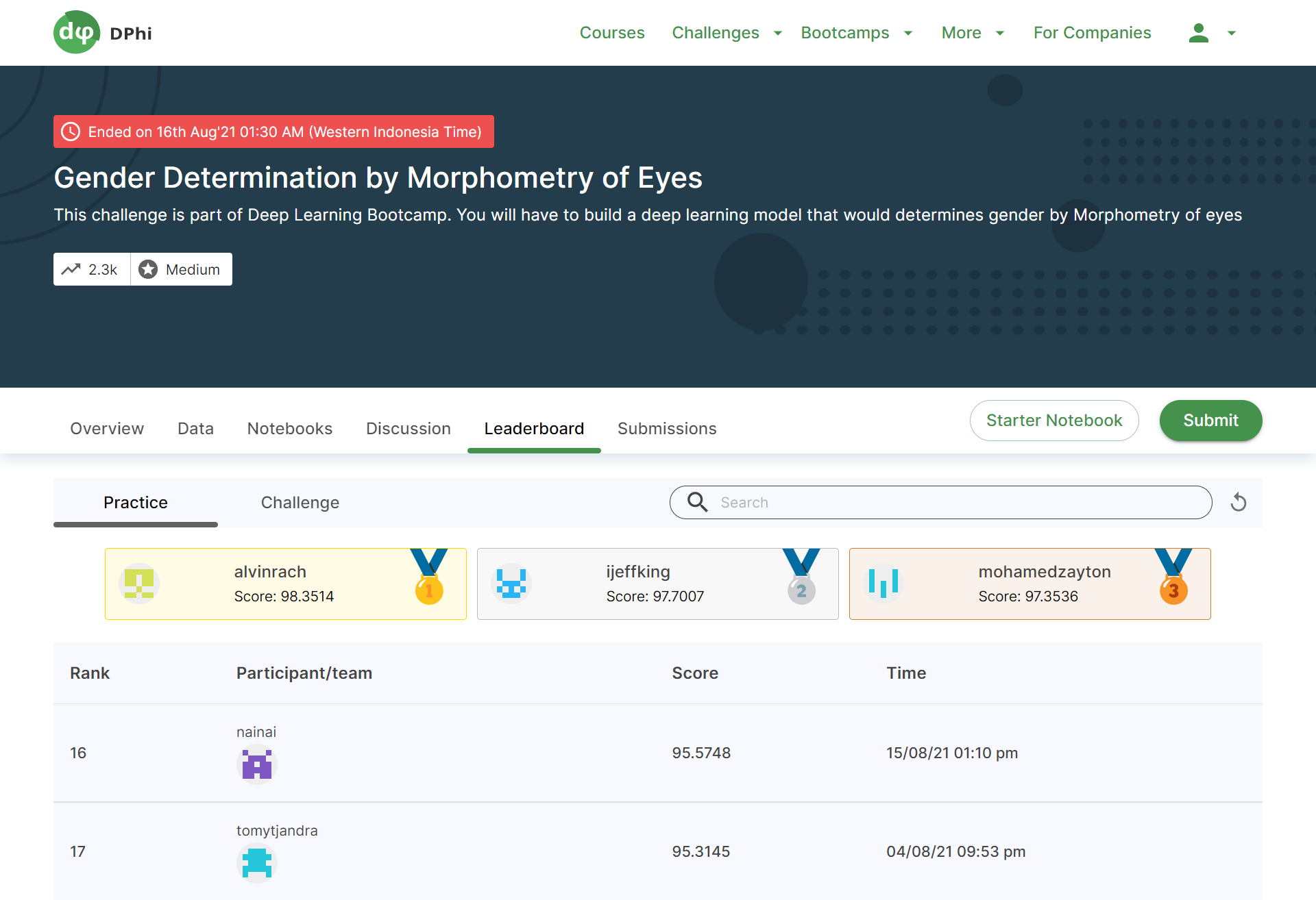
We are all set to make a submission. Let's head to the challenge page to make the submission.

Note: Placed 17th out of 118 submission, with model accuracy of 95.3145%