Convolutional Neural Network (CNN) for Casting Product Quality Inspection
Workflow on building a CNN model in Keras to classify whether a top-view image of casted submersible pump impeller is defect or ok. Data augmentation technique is applied to further improve model performance and generalization.
- Introduction
- Import Libraries
- Load the Images
- Visualize the Image
- Training the Network
- Testing on Unseen Images
- Conclusion
Introduction
Casting is a manufacturing process in which liquid material is poured into a mold to solidify. Many types of defects or unwanted irregularities can occur during this process. The industry has its quality inspection department to remove defective products from the production line, but this is very time consuming since it is carried out manually. Furthermore, there is a chance of misclassifying due to human error, causing rejection of the whole product order.
In this post, let us build a model by training top-view images of a casted submersible pump impeller using a Convolutional Neural Network (CNN) so that it can distinguish accurately between defect from the ok one.
We will break down into several steps:
-
Load the images and apply the data augmentation technique
-
Visualize the images
-
Training with validation: define the architecture, compile the model, model fitting and evaluation
-
Testing on unseen images
-
Make a conclusion
import pandas as pd
import numpy as np

# visualization
import matplotlib.pyplot as plt
import seaborn as sns
sns.set()

# neural network model
from keras.callbacks import ModelCheckpoint
from keras.layers import *
from keras.models import Sequential, load_model
from keras.preprocessing.image import ImageDataGenerator

# evaluation
from sklearn.metrics import confusion_matrix, classification_report
Load the Images
Here is the structure of our folder containing image data:
casting_data
├───test
│   ├───def_front
│   └───ok_front
└───train
    ├───def_front
    └───ok_front
The folder casting_data consists of two subfolders test and train in which each of them has another subfolder: def_front and ok_front denoting the class of our target variable. The images inside train will be used for model fitting and validation, while test will be used purely for testing the model performance on unseen images.
Data Augmentation
We apply on-the-fly data augmentation, a technique to expand the training dataset size by creating a modified version of the original image which can improve model performance and the ability to generalize. This can be achieved by using ImageDataGenerator provided by keras with the following parameters:
-
rotation_range: Degree range for random rotations. We choose 360 degrees since the product is a round object. -
width_shift_range: Fraction range of the total width to be shifted. -
height_shift_range: Fraction range of the total height to be shifted. -
shear_range: Degree range for random shear in a counter-clockwise direction. -
zoom_range: Fraction range for random zoom. -
horizontal_flipandvertical_flipare set toTruefor randomly flip image horizontally and vertically. -
brightness_range: Fraction range for picking a brightness shift value.
Other parameters:
-
rescale: Rescale the pixel values to be in range 0 and 1. -
validation_split: Reserve 20% of the training data for validation, and the rest 80% for model fitting.
train_generator = ImageDataGenerator(rotation_range=360,
                                     width_shift_range=0.05,
                                     height_shift_range=0.05,
                                     shear_range=0.05,
                                     zoom_range=0.05,
                                     horizontal_flip=True,
                                     vertical_flip=True,
                                     brightness_range=[0.75, 1.25],
                                     rescale=1./255,
                                     validation_split=0.2)
We define another set of value for the flow_from_directory parameters:
-
IMAGE_DIR: The directory where the image data is stored. -
IMAGE_SIZE: The dimension of the image (300 px by 300 px). -
BATCH_SIZE: Number of images that will be loaded and trained at one time. -
SEED_NUMBER: Ensure reproducibility. -
color_mode="grayscale": Treat our image with only one channel color. -
class_modeandclassesdefine the target class of our problem. In this case, we denote thedefectclass as positive (1), andokas a negative class. -
shuffle=Trueto make sure the model learns thedefectandokimages alternately.
IMAGE_DIR = "/kaggle/input/real-life-industrial-dataset-of-casting-product/casting_data/"
IMAGE_SIZE = (300, 300)
BATCH_SIZE = 64
SEED_NUMBER = 123

gen_args = dict(target_size=IMAGE_SIZE,
                color_mode="grayscale",
                batch_size=BATCH_SIZE,
                class_mode="binary",
                classes={"ok_front": 0, "def_front": 1},
                shuffle=True,
                seed=SEED_NUMBER)

train_dataset = train_generator.flow_from_directory(directory=IMAGE_DIR + "train",
                                                    subset="training", **gen_args)
validation_dataset = train_generator.flow_from_directory(directory=IMAGE_DIR + "train",
                                                         subset="validation", **gen_args)
test_generator = ImageDataGenerator(rescale=1./255)
test_dataset = test_generator.flow_from_directory(directory=IMAGE_DIR + "test",
                                                  **gen_args)
image_data = [{"data": typ,
               "class": name.split('/')[0],
               "filename": name.split('/')[1]}
              for dataset, typ in zip([train_dataset, validation_dataset, test_dataset], ["train", "validation", "test"])
              for name in dataset.filenames]
image_df = pd.DataFrame(image_data)
data_crosstab = pd.crosstab(index=image_df["data"],
                            columns=image_df["class"],
                            margins=True,
                            margins_name="Total")
data_crosstab
total_image = data_crosstab.iloc[-1, -1]
ax = data_crosstab.iloc[:-1, :-1].T.plot(kind="bar", stacked=True, rot=0)

percent_val = []

for rect in ax.patches:
    height = rect.get_height()
    width = rect.get_width()
    percent = 100*height/total_image

    ax.text(rect.get_x() + width - 0.25,
            rect.get_y() + height/2,
            int(height),
            ha='center',
            va='center',
            color="white",
            fontsize=10)

    ax.text(rect.get_x() + width + 0.01,
            rect.get_y() + height/2,
            "{:.2f}%".format(percent),
            ha='left',
            va='center',
            color="black",
            fontsize=10)

    percent_val.append(percent)

handles, labels = ax.get_legend_handles_labels()
ax.legend(handles=handles, labels=labels)

percent_def = sum(percent_val[::2])
ax.set_xticklabels(["def_front\n({:.2f} %)".format(
    percent_def), "ok_front\n({:.2f} %)".format(100-percent_def)])
plt.title("IMAGE DATA PROPORTION", fontsize=15, fontweight="bold")
plt.show()
We will proceed to the next step, since the proportion of data can be considered as balanced.
mapping_class = {0: "ok", 1: "defect"}

def visualizeImageBatch(dataset, title):
    images, labels = next(iter(dataset))
    images = images.reshape(BATCH_SIZE, *IMAGE_SIZE)
    fig, axes = plt.subplots(8, 8, figsize=(16, 16))

    for ax, img, label in zip(axes.flat, images, labels):
        ax.imshow(img, cmap="gray")
        ax.axis("off")
        ax.set_title(mapping_class[label], size=20)

    plt.tight_layout()
    fig.suptitle(title, size=30, y=1.05, fontweight="bold")
    plt.show()

    return images
train_images = visualizeImageBatch(
    train_dataset,
    "FIRST BATCH OF THE TRAINING IMAGES\n(WITH DATA AUGMENTATION)")
test_images = visualizeImageBatch(
    test_dataset,
    "FIRST BATCH OF THE TEST IMAGES\n(WITHOUT DATA AUGMENTATION)")
img = np.squeeze(train_images[4])[75:100, 75:100]

fig = plt.figure(figsize=(15, 15))
ax = fig.add_subplot(111)
ax.imshow(img, cmap="gray")
ax.axis("off")

w, h = img.shape
for x in range(w):
    for y in range(h):
        value = img[x][y]
        ax.annotate("{:.2f}".format(value), xy=(y, x),
                    horizontalalignment="center",
                    verticalalignment="center",
                    color="white" if value < 0.4 else "black")
These are the example of values that we are going to feed into our CNN architecture.
Training the Network
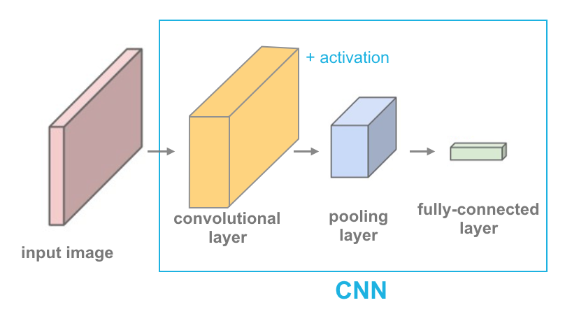
As mentioned earlier, we are going to train a CNN model to classify the casting product image. CNN is used as an automatic feature extractor from the images so that it can learn how to distinguish between defect and ok casted products. It effectively uses the adjacent pixel to downsample the image and then use a prediction (fully-connected) layer to solve the classification problem. This is a simple illustration by Udacity on how the layers are arranged sequentially:

Define Architecture
Here is the detailed architecture that we are going to use:
-
First convolutional layer: consists of 32
filterswithkernel_sizematrix 3 by 3. Using 2-pixelstridesat a time, reduce the image size by half. -
First pooling layer: Using max-pooling matrix 2 by 2 (
pool_size) and 2-pixelstridesat a time further reduce the image size by half. -
Second convolutional layer: Just like the first convolutional layer but with 16
filtersonly. - Second pooling layer: Same as the first pooling layer.
- Flattening: Convert two-dimensional pixel values into one dimension, so that it is ready to be fed into the fully-connected layer.
-
First dense layer + Dropout: consists of 128
unitsand 1 bias unit. Dropout ofrate20% is used to prevent overfitting. -
Second dense layer + Dropout: consists of 64
unitsand 1 bias unit. Dropout ofrate20% is also used to prevent overfitting. -
Output layer: consists of only one
unitandactivationis a sigmoid function to convert the scores into a probability of an image beingdefect.
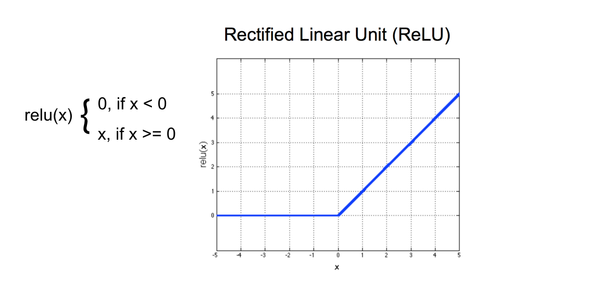
For every layer except output layer, we use Rectified Linear Unit (ReLU) activation function as follow:

model = Sequential(
    [
        # First convolutional layer
        Conv2D(filters=32,
               kernel_size=3,
               strides=2,
               activation="relu",
               input_shape=IMAGE_SIZE + (1, )),

        # First pooling layer
        MaxPooling2D(pool_size=2,
                     strides=2),

        # Second convolutional layer
        Conv2D(filters=16,
               kernel_size=3,
               strides=2,
               activation="relu"),

        # Second pooling layer
        MaxPooling2D(pool_size=2,
                     strides=2),

        # Flattening
        Flatten(),

        # Fully-connected layer
        Dense(128, activation="relu"),
        Dropout(rate=0.2),

        Dense(64, activation="relu"),
        Dropout(rate=0.2),

        Dense(1, activation="sigmoid")
    ]
)

model.summary()
model.compile(optimizer="adam",
              loss="binary_crossentropy",
              metrics=["accuracy"])
For each epoch, batch_size $\times$ steps_per_epoch images will be fed into our CNN architecture. In this case, we specify the steps_per_epoch to be 150 so for each epoch 64 * 150 = 9600 augmented images from the training dataset will be fed. We let the model train for 25 epochs.
By using ModelCheckpoint, the best model will be automatically saved if the current val_loss is lower than the previous one.
STEPS = 150

checkpoint = ModelCheckpoint("cnn_casting_inspection_model.hdf5",
                             verbose=1,
                             save_best_only=True,
                             monitor="val_loss")

model.fit_generator(generator=train_dataset,
                    validation_data=validation_dataset,
                    steps_per_epoch=STEPS,
                    epochs=25,
                    validation_steps=STEPS,
                    callbacks=[checkpoint],
                    verbose=1)
plt.subplots(figsize=(8, 6))
sns.lineplot(data=pd.DataFrame(
    model.history.history,
    index=range(1, 1+len(model.history.epoch))))
plt.title("TRAINING EVALUATION", fontweight="bold", fontsize=20)
plt.xlabel("Epochs")
plt.ylabel("Metrics")

plt.legend(labels=['val loss', 'val accuracy', 'train loss', 'train accuracy'])
plt.show()
train loss and val loss simultaneously dropped towards zero. Also, both train accuracy and val accuracy increases towards 100%.
best_model = load_model("/kaggle/working/cnn_casting_inspection_model.hdf5")
y_pred_prob = best_model.predict_generator(generator=test_dataset, verbose=1)
The output of the prediction is in the form of probability. We use THRESHOLD = 0.5 to separate the classes. If the probability is greater or equal to the THRESHOLD, then it will be classified as defect, otherwise ok.
THRESHOLD = 0.5
y_pred_class = (y_pred_prob >= THRESHOLD).reshape(-1,)
y_true_class = test_dataset.classes[test_dataset.index_array]

pd.DataFrame(
    confusion_matrix(y_true_class, y_pred_class),
    index=[["Actual", "Actual"], ["ok", "defect"]],
    columns=[["Predicted", "Predicted"], ["ok", "defect"]],
)
print(classification_report(y_true_class, y_pred_class, digits=4))
On test dataset, the model achieves a very good result as follow:
- Accuracy: 99.44%
- Recall: 99.78%
- Precision: 99.34%
- F1 score: 99.56%
defect product is misclassified as ok. This can cause the whole order to be rejected and create a big loss for the company. Therefore, in this case, we prioritize Recall over Precision. But if we take into account the cost of re-casting a product, we have to minimize the case of False Positive also, where the ok product is misclassified as defect. Therefore we can prioritize the F1 score which combines both Recall and Precision.
images, labels = next(iter(test_dataset))
images = images.reshape(BATCH_SIZE, *IMAGE_SIZE)
fig, axes = plt.subplots(4, 4, figsize=(16, 16))

for ax, img, label in zip(axes.flat, images, labels):
    ax.imshow(img, cmap="gray")
    true_label = mapping_class[label]

    [[pred_prob]] = best_model.predict(img.reshape(1, *IMAGE_SIZE, -1))
    pred_label = mapping_class[int(pred_prob >= THRESHOLD)]

    prob_class = 100*pred_prob if pred_label == "defect" else 100*(1-pred_prob)

    ax.set_title(f"TRUE LABEL: {true_label}", fontweight="bold", fontsize=18)
    ax.set_xlabel(f"PREDICTED LABEL: {pred_label}\nProb({pred_label}) = {(prob_class):.2f}%",
                  fontweight="bold", fontsize=15,
                  color="blue" if true_label == pred_label else "red")

    ax.set_xticks([])
    ax.set_yticks([])

plt.tight_layout()
fig.suptitle("TRUE VS PREDICTED LABEL FOR 16 RANDOM TEST IMAGES",
             size=30, y=1.03, fontweight="bold")
plt.show()
Since the proportion of correctly classified images is very large, let's also visualize the misclassified only.
misclassify_pred = np.nonzero(y_pred_class != y_true_class)[0]

fig, axes = plt.subplots(2, 2, figsize=(8, 8))

for ax, batch_num, image_num in zip(axes.flat, misclassify_pred // BATCH_SIZE, misclassify_pred % BATCH_SIZE):
    images, labels = test_dataset[batch_num]
    img = images[image_num]
    ax.imshow(img.reshape(*IMAGE_SIZE), cmap="gray")

    true_label = mapping_class[labels[image_num]]
    [[pred_prob]] = best_model.predict(img.reshape(1, *IMAGE_SIZE, -1))
    pred_label = mapping_class[int(pred_prob >= THRESHOLD)]

    prob_class = 100*pred_prob if pred_label == "defect" else 100*(1-pred_prob)

    ax.set_title(f"TRUE LABEL: {true_label}", fontweight="bold", fontsize=18)
    ax.set_xlabel(f"PREDICTED LABEL: {pred_label}\nProb({pred_label}) = {(prob_class):.2f}%",
                  fontweight="bold", fontsize=15,
                  color="blue" if true_label == pred_label else "red")

    ax.set_xticks([])
    ax.set_yticks([])

plt.tight_layout()
fig.suptitle(f"MISCLASSIFIED TEST IMAGES ({len(misclassify_pred)} out of {len(y_true_class)})",
             size=20, y=1.03, fontweight="bold")
plt.show()
Out of 715 test images, only 4 images are being misclassified.
Conclusion
By using CNN and on-the-fly data augmentation, the performance of our model in training, validation, and test images is almost perfect, reaching 98-99% accuracy and F1 score. We can utilize this model by embedding it into a surveillance camera where the system can automatically separate defective product from the production line. This method surely can reduce human error and human resources on manual inspection, but it still needs supervision from human since the model is not 100% correct at all times.